Introduction
In The Name of GOD
Ali Pilehvar Meibody
Presentation for Prof. Malek Naderi
At Gamlab , 16 April 2024
PyGamLab Library
![]()
Importance of python
Importance of libraries in Python programming
What is PyGamlab
PyGamLab is a scientific Python library developed for researchers, engineers, and students who need access to fundamental constants, conversion tools, engineering formulas, and data analysis utilities. The package is designed with simplicity, clarity, and usability in mind.
PyGAMLab stands for Python GAMLAb tools, a collection of scientific tools and functions developed at the GAMLab (Graphene and Advanced Material Laboratory) by Ali Pilehvar Meibody under the supervision of Prof. Malek Naderi at Amirkabir University of Technology (AUT).
Author: Ali Pilehvar Meibody
Supervisor: Prof. Malek Naderi
Affiliation: GAMLab, Amirkabir University of Technology (AUT)
📦 Modules
PyGAMLab is composed of four core modules, each focused on a specific area of scientific computation:
🔹 Constants.py
This module includes a comprehensive set of scientific constants used in physics, chemistry, and engineering.
Examples:
Planck’s constant
Boltzmann constant
Speed of light
Universal gas constant
Density of Metals
Tm of Metals
And many more…
🔹 Convertors.py
FirstUnit_To_SecondUnit()Examples:
Kelvin_To_Celsius(k)Celsius_To_Kelvin(c)Meter_To_Foot(m)…and many more standard conversions used in science and engineering.
🔹 Functions.py
This module provides a wide collection of scientific formulas and functional tools commonly used in engineering applications.
Examples:
Thermodynamics equations
Mechanical stress and strain calculations
Fluid dynamics formulas
General utility functions
🔹 Data_Analysis.py
Provides tools for working with data, either from a file path or directly from a DataFrame.
Features include:
Reading and preprocessing datasets
Performing scientific calculations
Creating visualizations (e.g., line plots, scatter plots, histograms)
📦 Requirements
To use PyGamLab, make sure you have the following Python packages installed:
numpypandasscipymatplotlibseabornscikit-learn
You can install all dependencies using:
pip install numpy pandas scipy matplotlib seaborn scikit-learn
How to install 🚀
To install PyGAMLab via pip:
pip install pygamlab
or
git clone https://github.com/APMaii/pygamlab.git
How to Import
[3]:
import PyGamLab


#PyGamLab.Constants.


#PyGamLab.Convertors.


#PyGamLab.Functions.


#PyGamLab.Data_Analysis.

#----or better way-----

import PyGamLab.Constants as gamcons
import PyGamLab.Convertors as gamconv
import PyGamLab.Functions as gamfunc
import PyGamLab.Data_Analysis as gamdat
Constants.
This module includes a comprehensive set of scientific constants used in physics, chemistry, and engineering.
[5]:
import PyGamLab.Constants as gamcons

gamcons.K_boltzman
[5]:
1.380649e-23
[7]:
gamcons.h_plank
[7]:
6.62607015e-34
[9]:
gamcons.stefan_boltzmann_constant
[9]:
5.67e-08
[11]:
gamcons.h_plank
[11]:
6.62607015e-34
[13]:
#fluid dynamics-----------
# Dynamic Viscosity of air at 20°C (Pa·s)
print(gamcons.mu_air_20C)

print(gamcons.Re_laminar)

print(gamcons.Re_turbulent)

#heat transfer-----------

print(gamcons.thermal_conductivity_air)

print(gamcons.specific_heat_water)
1.81e-05
2000
4000
0.0262
4.18
[19]:
#----geometric

print(gamcons.earth_mass)
print(gamcons.earth_volume)

#---Thermodynamic---

print(gamcons.gibbs_free_energy_water)

print(gamcons.avogadro_constant)

#---physic

print(gamcons.electron_mass)
print(gamcons.neutron_mass)
5.972e+24
1083210000000.0
-237.13
6.02214076e+23
9.10938356e-31
1.675e-27
[21]:
#---material properties


print(gamcons.ELEMENTS_Tm['Al'])
print(gamcons.ELEMENTS_Tm['Cu'])
print(gamcons.ELEMENTS_Tm['Ti'])
print(gamcons.ELEMENTS_Tm['Si'])


print(gamcons.ELEMENTS_DENSITY['H'])
print(gamcons.ELEMENTS_DENSITY['He'])

print(gamcons.ELEMENTS_DENSITY['Al'])
print(gamcons.ELEMENTS_DENSITY['Cu'])
print(gamcons.ELEMENTS_DENSITY['Ti'])
print(gamcons.ELEMENTS_DENSITY['Si'])


print(gamcons.electronegativity['H'])
print(gamcons.electronegativity['Li'])
print(gamcons.electronegativity['Cl'])


print(gamcons.atomic_radius['H'])
print(gamcons.atomic_radius['Li'])
print(gamcons.atomic_radius['Cl'])


print(gamcons.thermal_conductivity['Al'])
print(gamcons.thermal_conductivity['Si'])
print(gamcons.thermal_conductivity['Fe'])


print(gamcons.electrical_conductivity['Al'])
print(gamcons.electrical_conductivity['Si'])
print(gamcons.electrical_conductivity['Fe'])
933.47
1357.77
1941
1687
8.988e-05
0.0001785
2.7
8.96
4.54
2.3296
2.2
0.98
3.16
31
128
102
237
149
80.2
37.7
0.000156
10
[29]:
#----or you can have your element------


h=gamcons.H_Type()
print(h.symbol)
print(h.atomic_number)
print(h.density)


si=gamcons.Si_Type()
print(si.symbol)
print(si.atomic_number)
print(si.density)
print(si.melting_point)
print(si.thermal_conductivity )
print(si.electrical_conductivity)


al=gamcons.Al_Type()
print(al.symbol)
print(al.atomic_number)
print(al.density)
print(al.melting_point)
print(al.thermal_conductivity )
print(al.electrical_conductivity)
H
1
8.988e-05
Si
14
2.329
1687
149
13800000.0
Al
13
2.7
933.47
235
37700000.0
Convertors.py
[27]:
#-------Convertors-------
import PyGamLab.Convertors as gamconv
#from simple
#it is readable
[27]:
print(gamconv.Angstrom_To_Meter(1))
1e-10
[29]:
print(gamconv.Angstrom_To_Nanometer(10))
1.0
[31]:
print(gamconv.Nanometer_To_Angstrom(10))
100
[124]:
print(gamconv.Inch_To_Centimeter(1))
2.54
[126]:
print(gamconv.Joules_To_Calories(1))
0.2390057361376673
[128]:
print(gamconv.Celcius_To_Kelvin(25))
298.15
[130]:
print(gamconv.Kelvin_to_Celcius(300))
26.850000000000023
[132]:
print(gamconv.Centigrade_To_Fahrenheit(25))
77.0
[134]:
print(gamconv.LightYear_To_KiloMeter(1))
9460730472801.1
[138]:
print(gamconv.Atmosphere_To_Pascal(1))
101325.0
[142]:
print(gamconv.Coulomb_To_Electron_volt(1))
6.24e+18
[144]:
print(gamconv.Watt_To_Horsepower(1))
1.341022e-03
[146]:
print(gamconv.Newton_TO_Pound_Force(1))
0.22480894291071968
Functions.py
[150]:
import PyGamLab.Functions as gamfunc

gamfunc.Bouyancy_Force(1000, 0.01)  # Water (kg/m³), 0.01 m³ (10L object)
[150]:
98.10000000000001
[152]:
gamfunc.coulombs_law(charge1=1e-6, charge2=2e-6, distance=0.05)
[152]:
7.189999999999998
[156]:
gamfunc.Electrical_Resistance(v=12, i=2)
[156]:
6.0
[158]:
gamfunc.Activation_Energy(k=2e5, k0=1e13, T=298)
[158]:
43923.66981946115
[160]:
gamfunc.root_degree2(a=1, b=-3, c=2)
[160]:
2.0
[31]:
gamfunc.Transient_Heat_Conduction_Semi_Infinite_Solid(T_s=100, T_i=25, alpha=1e-5, x=0.01, t=60)
[31]:
82.96224945133356
[33]:
# Define G(T) for two phases
G_alpha = lambda T: -10000 + 5*T
G_beta = lambda T: -9000 + 4.8*T

print(gamfunc.predict_phase_from_gibbs(G_alpha, G_beta, 800))  # Returns which is stable
Phase 1
Data Analysis
[35]:
import pandas as pd
import numpy as np
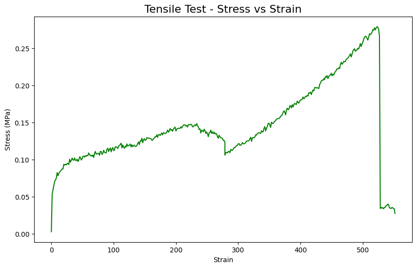
Tensile test
[37]:
fname2='/Users/apm/Desktop/PyGamLab/data_examples/Tensile test.xlsx'
data2=pd.read_excel(fname2)
gamdat.Tensile_Analysis(data2,application='plot-stress')
[39]:
fname2='/Users/apm/Desktop/PyGamLab/data_examples/Tensile test.xlsx'
data2=pd.read_excel(fname2)
gamdat.Tensile_Analysis(data2,application='UTS')
Ultimate Tensile Strength (UTS): 0.28 MPa
[39]:
np.float64(0.2789497)
<Figure size 6000x3600 with 0 Axes>
[43]:
fname2='/Users/apm/Desktop/PyGamLab/data_examples/Tensile test.xlsx'
data2=pd.read_excel(fname2)
gamdat.Tensile_Analysis(data2,application='Young Modulus')
Young’s Modulus (E): 0.00 MPa
[43]:
np.float64(0.0009208410039255529)
<Figure size 6000x3600 with 0 Axes>
[45]:
fname2='/Users/apm/Desktop/PyGamLab/data_examples/Tensile test.xlsx'
data2=pd.read_excel(fname2)
gamdat.Tensile_Analysis(data2,application='Fracture Stress')
Fracture Stress: 0.03 MPa
[45]:
np.float64(0.02765656)
<Figure size 6000x3600 with 0 Axes>
[47]:
fname2='/Users/apm/Desktop/PyGamLab/data_examples/Tensile test.xlsx'
data2=pd.read_excel(fname2)
gamdat.Tensile_Analysis(data2,application='Strain at break')
Strain at Break: 551.6282
[47]:
np.float64(551.6282)
<Figure size 6000x3600 with 0 Axes>
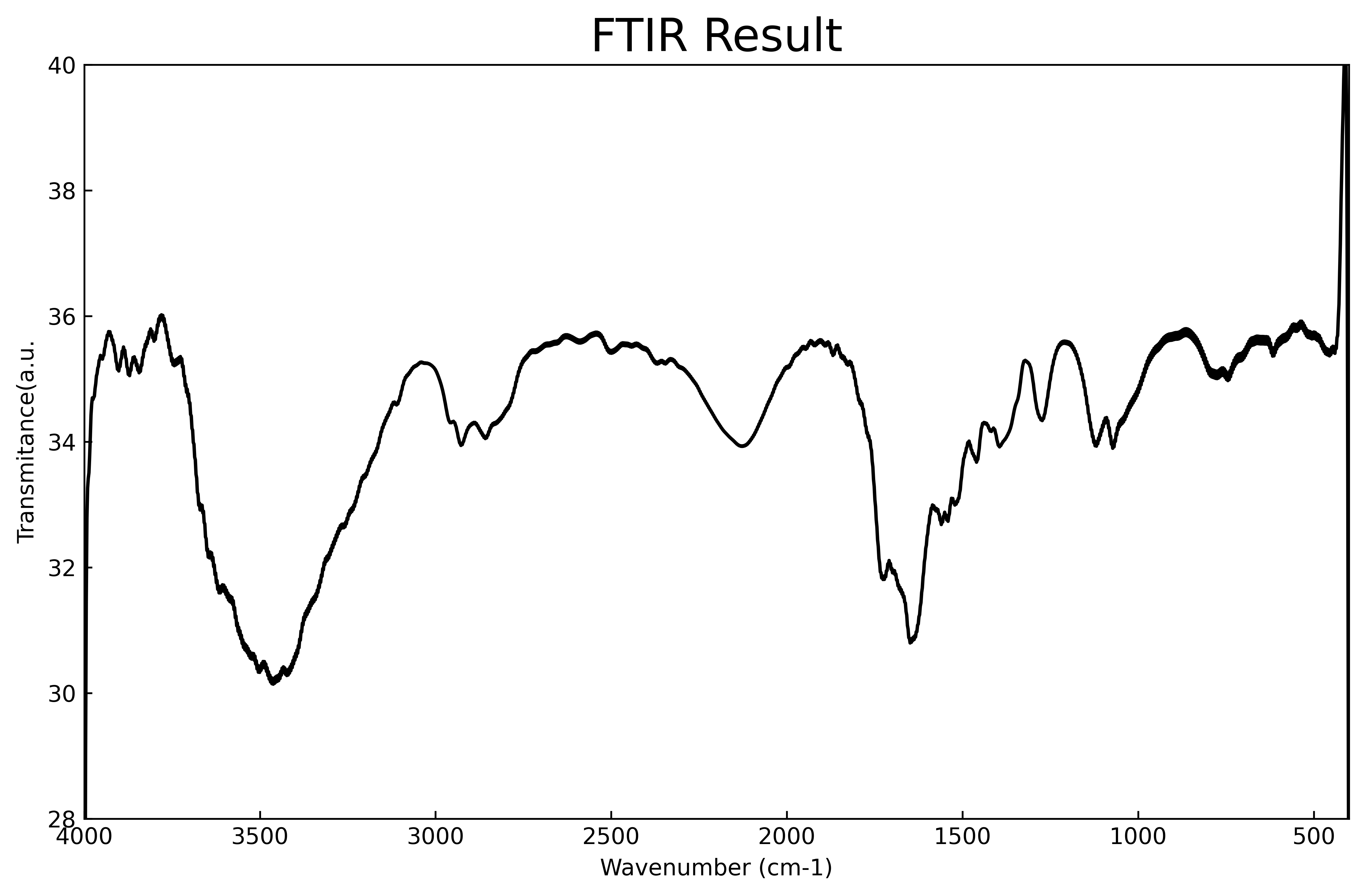
FTIR
[49]:
fname1='/Users/apm/Desktop/PyGamLab/data_examples/FTIR-B.txt'
data1=open(fname1,'r')
data1=pd.read_csv(fname1)
[51]:
gamdat.FTIR(data1,application='plot')
[53]:
gamdat.FTIR(data1,application='peak')
[53]:
(array([  36,  114,  498,  755, 1086, 1389, 1447, 1627, 1795, 1861]),
 {'prominences': array([ 0.701443,  5.877992,  1.327134,  4.946387,  1.698551,  0.959503,
          1.705757,  0.826016,  0.552433, 18.253715]),
  'left_bases': array([   0,    0,  279,  279,  971, 1219, 1219,  279,  279,    0]),
  'right_bases': array([  67,  279,  556, 1219, 1219, 1414, 1518, 1688, 1838, 1867])})
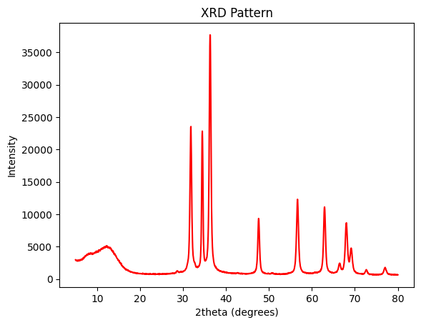
XRD
[55]:
XRD=pd.read_excel('/Users/apm/Desktop/PyGamLab/data_examples/ZnO.xlsx')
[108]:
gamdat.XRD_ZnO(XRD,'plot')
[110]:
fwhm = gamdat.XRD_ZnO(XRD, 'FWHM')
[112]:
crystal_size = gamdat.XRD_ZnO(XRD, 'Scherrer')
[114]:
print(fwhm,crystal_size)
4.800000000000001 17.33820358543292
Development in Version.2
Integration with experimental data
including new simulation tools (Molecular dynamic, Quantum DFT , FEM)
Including automated Machine learning for training the experimental data
Transfer Learning : including engineering pre-trained model
Further Information
Github source : https://github.com/APMaii/pygamlab.git
PYPI : https://pypi.org/project/PyGamLab/
pip install pygamlab