Getting Started with PyGamLab V2

It provides tools for:

Building and visualizing atomic and nanostructures
Connecting to material databases
Loading and fine-tuning pre-trained AI models
Analyzing experimental data
Using fundamental constants, conversion utilities, and engineering formulas

This guide will help you install PyGamLab and explore its tools, functions, and classes step by step. You can either follow the tutorial from start to finish or click the sections in the table of contents to jump directly to the topic of interest.

Table of Contents¶

0. Overview of PyGamLab
1. How to Install
2. Constants & Converters
3. Functions
4. Nano Structures
5. Databases
6. Nano Data Analysis
7. Nano AI – Pre-trained Models
8. Appendix A: Using NumPy
9. Appendix B: Using Pandas
10. Appendix C: Using scikit-learn

0. Overview of PyGamLab¶

PyGamLab is a comprehensive Python library designed to empower researchers, engineers, and students working in materials science and nanotechnology. It combines scientific computing, AI, and domain-specific tools to streamline workflows from data analysis to simulation and modeling.

In this section, we provide a detailed overview of the main capabilities of PyGamLab and how they can support your research and projects.

Key Features¶

PyGamLab allows you to generate, manipulate, and visualize atomic
and nanostructures with ease.
- Create crystalline lattices, nanoparticles, and alloy structures.
- Visualize structures in 2D and 3D using built-in plotting tools.
- Export structures to common file formats for simulation software.
- Modify structures dynamically to study defects, substitutions, or
surface effects.

This feature is especially useful for simulation preparation, nanostructure design, and teaching purposes.

Access and query physical, chemical, and thermodynamic properties
of materials from integrated databases.
- Retrieve element properties, compound data, and experimental
results.
- Query materials using properties, composition, or structural
parameters.
- Integrate with local or online databases for automated data
retrieval.

This functionality reduces manual data collection, making your workflow faster and more reproducible.

PyGamLab comes with tools to load, fine-tune, and apply pre-trained
AI models for materials research.
- Predict material properties from structure or composition.
- Fine-tune models with your own datasets.
- Perform advanced analysis such as clustering, regression, or
classification for experimental and simulation data.

The AI module allows you to leverage state-of-the-art machine learning without needing to implement models from scratch.

Analyze experimental or simulation datasets efficiently with
PyGamLab’s nano-focused data analysis tools.
- Import, clean, and preprocess datasets from various sources.
- Compute statistical and physical descriptors relevant to
nanomaterials.
- Generate visualizations such as histograms, scatter plots, and
heatmaps.
- Perform advanced analyses like correlation studies, regression, or
pattern recognition.

These tools are tailored to nanoscience and materials data, providing high-level insights with minimal code.

PyGamLab includes a set of utility functions and constants for
scientific computation:
- Access fundamental physical constants.
- Perform unit conversions with ease (e.g., nm → m, eV → J).
- Use built-in engineering formulas for common calculations in
materials science.

These utilities reduce boilerplate code, ensuring calculations are accurate and consistent.

How This Tutorial Helps You¶

In this tutorial, we will walk through all the main PyGamLab modules with practical examples:

Start with installation and setup.
Explore constants, converters, and utility functions.
Learn to work with datasets using functions and analysis tools.
Build and visualize nanostructures for simulations.
Use AI models for prediction and advanced data analysis.

By the end of this tutorial, you will have a clear understanding of PyGamLab’s capabilities and how to apply them to your research projects or coursework in materials science and nanotechnology.

1. How to Install¶

Before you can use PyGamLab’s powerful tools, classes, and functions, you need to install the library. Like most Python libraries, PyGamLab can be installed using pip, Python’s package manager.

Step 1: Open Your Command Line Interface¶

Windows: Press Win + R, type cmd, and press Enter to open the Command Prompt.
MacOS: Open Terminal from Applications → Utilities.
Linux: Open your preferred terminal application.

Once you have your terminal open, you can proceed with the installation.

Step 2: Install PyGamLab¶

You can install the latest stable version of PyGamLab using:

pip install pygamlab

Or, if you want the latest development version directly from GitHub:

pip install git+https://github.com/APMaii/pygamlab.git

Tip: It is recommended to use a virtual environment to avoid conflicts with other Python packages. You can create one using:

python -m venv myenv
source myenv/bin/activate   # On MacOS/Linux
myenv\Scripts\activate      # On Windows

Step 3: Verify the Installation¶

After installation, check if PyGamLab is correctly installed by running:

import pygamlab
print(pygamlab.__version__)

If this prints the version number without any errors, you’re all set and ready to start using PyGamLab.

Installing pip (if needed)¶

If you do not have pip installed yet, you can install it using the following command (requires Python 3.4+):

python -m ensurepip --upgrade

Alternatively, follow the official pip installation guide here: https://pip.pypa.io/en/stable/installation/

Once pip is installed, you can follow Step 2 to install PyGamLab.

2. Constants & Converters¶

One of the core ideas of PyGamLab V1 was to provide a centralized place for constants and unit converters. This helps researchers, engineers, and students avoid repeatedly searching for values or hardcoding “magic numbers” in their code.

Why Constants & Converters Matter¶

Constants: These are predefined variables representing important physical, chemical, and engineering values. In PyGamLab, constants include:
- Formula constants
- Material properties
- Semiconductor properties
- Thermal, electrical, and mechanical properties
By using named constants instead of raw numbers, your code becomes more readable, maintainable, and easier to debug.
Converters: PyGamLab provides a collection of functions to convert units between different systems. This allows you to work seamlessly with various measurement units without manually calculating conversions every time.

How PyGamLab Implements This¶

All constants are stored in the Constants module, while conversion functions are grouped together in utility functions. This design ensures that:

You never need to memorize values or look them up repeatedly.
Your code is self-explanatory, as each constant has a meaningful name.
You can quickly switch units in calculations, making your experiments or simulations consistent and accurate.

Example Usage¶

from pygamlab.Constants import PhysicalConstants
from pygamlab.converters import unit_convert

# Accessing a constant
speed_of_light = PhysicalConstants.c
print(speed_of_light)  # 299792458 m/s

# Converting units
length_in_cm = unit_convert(1, from_unit="m", to_unit="cm")
print(length_in_cm)  # 100

With this approach, PyGamLab ensures that your code is clean, understandable, and scientifically accurate.

3. Functions¶

The Functions module in PyGamLab V1 is one of the most important modules for researchers, engineers, and students in materials science, nanotechnology, thermodynamics, and physics.

What is the Functions Module?¶

The Functions module is essentially a collection of ready-to-use scientific formulas. Instead of manually coding equations every time, you can use these functions to perform calculations related to:

Material properties
Thermodynamic processes
Crystallography
Electrostatics
Nano-scale phenomena

This module provides a reliable and tested set of formulas that are frequently used in scientific computing.

Purpose of the Functions Module¶

Save Time and Reduce Errors

Instead of implementing formulas yourself, you can rely on pre-built, tested functions. This reduces coding mistakes and ensures accurate calculations.
Improve Readability and Maintainability

Using descriptive function names like Coulombs_Law or Activation_Energy avoids “magic numbers” in your code and makes it easier to understand and debug.
Enable Rapid Prototyping

You can quickly integrate these functions into your simulations or experiments without worrying about the underlying math.
Consistency Across Projects

By using a standardized set of functions, your calculations remain consistent and reproducible across different projects or collaborators.

Advantages of Using the Functions Module¶

Scientifically accurate: All formulas are based on standard scientific principles.
Well-documented: Each function comes with parameter explanations and return values.
Interoperable: Works seamlessly with PyGamLab’s Constants, Converters, and AI modules.
Versatile: Functions cover a wide range of domains, from classical physics to nanomaterial properties.

Examples of Functions and Usage¶

The Activation Energy function calculates the energy required for a reaction to occur using the Arrhenius equation:

import math
from pygamlab.functions import Activation_Energy

k = 0.01   # rate constant at T
k0 = 1.0   # pre-exponential factor
T = 300    # temperature in Kelvin

Ea = Activation_Energy(k, k0, T)
print(f"Activation Energy: {Ea:.2f} J/mol")

The Bragg Law function calculates the diffraction angle of X-rays through a crystal lattice:

from pygamlab.functions import Bragg_Law

theta = Bragg_Law(h=1, k=1, l=1, a=0.5, y=0.154)
print(f"Diffraction angle: {theta:.2f}°")

This is useful for analyzing crystal structures or interpreting X-ray diffraction data.

The Debye Temperature function estimates the characteristic temperature of a solid material:

from pygamlab.functions import Calculate_Debye_Temperature

theta_D = Calculate_Debye_Temperature(velocity=5000, atomic_mass=63.55, density=8960, n_atoms=1)
print(f"Debye Temperature: {theta_D} K")

The Coulombs_Law function calculates the electrostatic force between two charges:

from pygamlab.functions import Coulombs_Law

F = Coulombs_Law(charge1=1e-6, charge2=2e-6, distance=0.01)
print(f"Electrostatic Force: {F:.4f} N")

Useful for nanostructure simulations, charge interaction analysis, and electrostatic modeling.

The Functions module is a core part of PyGamLab designed to make scientific computations faster, safer, and more readable. By providing a collection of well-documented formulas, this module allows users to focus on research and experimentation rather than coding routine equations. It works best when combined with Constants and Converters, forming a powerful toolkit for materials science and nanotechnology research.

4. Structures¶

At the heart of PyGamLab V2 lies the Structures module, designed specifically for nanotechnology and computational materials science. This module provides tools to create, manipulate, visualize, and export atomic and nano-scale structures.

With this module, you can generate:

0D materials (e.g., clusters or nanoparticles)
1D materials (e.g., nanowires)
2D materials (e.g., graphene sheets, monolayers)
Bulk structures (crystalline materials, lattices)

Each structure is represented as an object-oriented class, where every atom, bond, or unit has attributes (e.g., position, type, charge) and methods (e.g., translate, rotate, bond, calculate distances). This allows full control over building, modifying, and analyzing structures.

Once created, structures can be:

Adjusted and manipulated
Visualized using multiple engines
Converted to popular formats for other packages like ASE or Pymatgen
Exported for input to simulation software

Advantages of the Structures Module¶

Object-oriented design: Each atom or bond is a class instance with attributes and methods.
Supports all dimensions: Build 0D, 1D, 2D, or 3D bulk materials.
Integration with other tools: Convert structures to ASE or Pymatgen objects.
Powerful generators: Create complex structures with fewer lines of code compared to writing everything manually.
Visualization support: Multiple engines like Matplotlib, PyVista, or built-in software for real-time visualization.
Robust structure management: Includes readers, exporters, converters, and checkers for handling files and object formats.

Submodules Overview¶

The PrimAtom submodule defines the fundamental units of structures:

GAM_Atom: Represents a single atom.
GAM_Bond: Represents a bond between atoms.

These are the building blocks for all structures. With multiple GAM_Atom and GAM_Bond objects, you can create highly complex nanostructures.

The Generators submodule provides top-level classes built on ASE objects, allowing you to:

Create complex structures that would otherwise take 40+ lines of ASE code.
Automatically generate atomic arrangements and lattice patterns.
Perform operations on the structure after creation.

This is particularly useful for advanced material design and simulation setup.

The GAM_Architecture submodule focuses on core mathematical and scratch-built structures. It allows you to:

Build structures from scratch (e.g., graphene, nanotubes).
Use predefined geometric patterns for common materials.

It’s the foundation of the structures module.

The I/O submodule manages:

Read: Load structures in GAM_Atom format.
Export: Save structures for external software or simulations.
Conversion: Convert between ASE, Pymatgen, or GAM_Atom objects.
Checker: Identify the type and validity of your structure objects.

The Molecular_Visualized submodule (from GAMVIS) enables visualization of structures using multiple engines:

Matplotlib – basic plotting
PyVista – 3D interactive visualization
Built-in engine – opens a dedicated visualization software for real-time exploration

Example Usage¶

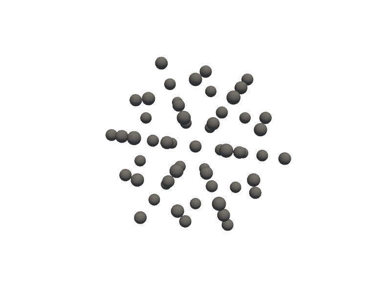
#Creation of Au nano cluster

#first from Generators import Nano_OneD_Builder claas
from PyGamLab.structures.Generators import Nano_ZeroD_Builder


#create one object from this object with specific parameters
builder=Nano_ZeroD_Builder(material="Au",
                        structure_type="nanocluster",
                        size=3, # or use noshells=3
                        noshells=3,
                        crystal_structure="fcc",
                        lattice_constant=4.08)

#now you have your object and you can utilize its methods
#you can add defects with add_defects method
#you can create alloys and .....
#but for now , juts you can get the atoms (which are from Primatom class)
my_atoms=builder.get_atoms()

#for visulization you can use Molecular_Visulizer class
from PyGamLab.structures.gamvis import Molecular_Visualizer

Molecular_Visualizer(my_atoms,format='efficient_plotly')
#also you can use other formats like 'ase', 'gamvis' and 'pyvista'

Visualizing 55 atoms using efficient_plotly format...

Molecular_Visualizer(my_atoms,format='pyvista')

Visualizing 55 atoms using pyvista format...

/Users/apm/anaconda3/envs/DL/lib/python3.10/site-packages/pyvista/jupyter/notebook.py:56: UserWarning:

Failed to use notebook backend:

No module named 'trame'

Falling back to a static output.

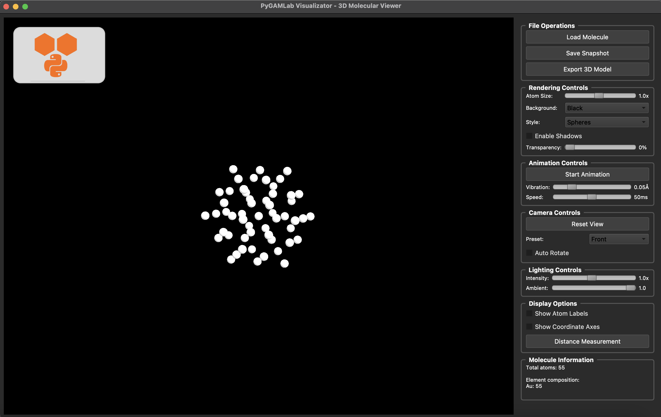
Molecular_Visualizer(my_atoms,format='gamvis')

Visualizing 55 atoms using gamvis format...
=== PyGAMLab Visualizator Debug Info ===
Python version: 3.10.13 | packaged by conda-forge | (main, Dec 23 2023, 15:35:25) [Clang 16.0.6 ]
PyQt5 version: 5.15.2
Platform: Darwin 24.3.0
Creating main window...
Loading 55 atoms...
Showing window...
Initializing VTK interactor...

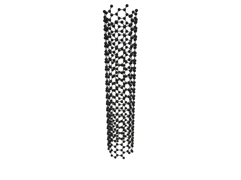
#also you can create One dimensional nanostructures like nanowires and nanotubes
from PyGamLab.structures.Generators import Nano_OneD_Builder

#You can create a carbon nanotube with length of 5.0 Angstrom and vacuum of 8.0 Angstrom
tube = Nano_OneD_Builder(material="C", structure_type="nanotube", length=5.0, vacuum=8.0)

#then you can use its methods like get_atoms to get the atoms object
tube_atoms = tube.get_atoms()

#for visulization you can use Molecular_Visulizer class
Molecular_Visualizer(tube_atoms, format='pyvista')

Visualizing 480 atoms using pyvista format...

/Users/apm/anaconda3/envs/DL/lib/python3.10/site-packages/pyvista/jupyter/notebook.py:56: UserWarning:

Failed to use notebook backend:

No module named 'trame'

Falling back to a static output.

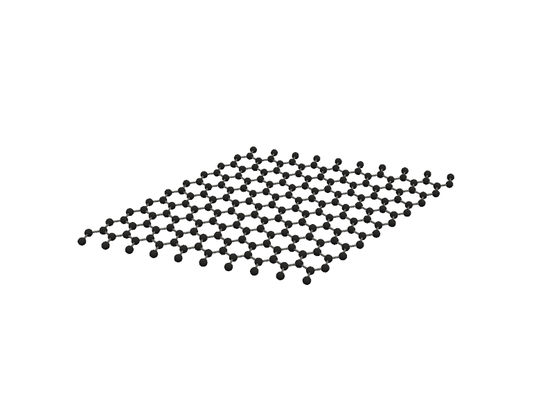
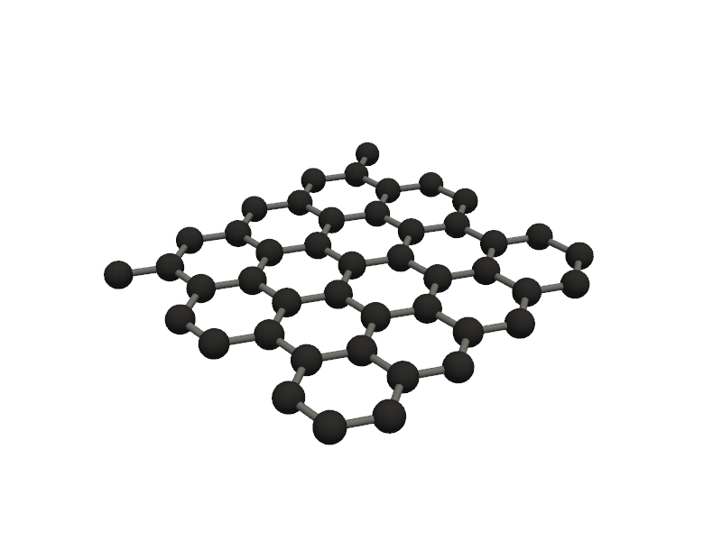
#Like ZeroD and OneD nanostructures, you can create TwoD nanostructures like nanosheets and nanoribbons
from PyGamLab.structures.Generators import Nano_TwoD_Builder
builder_graphene = Nano_TwoD_Builder(material="graphene", structure_type="nanosheet")

graphene_atoms = builder_graphene.get_atoms()

Molecular_Visualizer(graphene_atoms, format='pyvista')

Visualizing 200 atoms using pyvista format...

/Users/apm/anaconda3/envs/DL/lib/python3.10/site-packages/pyvista/jupyter/notebook.py:56: UserWarning:

Failed to use notebook backend:

No module named 'trame'

Falling back to a static output.

#aLSO, you can create advanced alloys using AdvancedAlloys class
from PyGamLab.structures.Generators import AdvancedAlloys
alloy9 = AdvancedAlloys(
elements=["Au", "C"],
fractions=[0.6, 0.4],
metadata={"project": "test_alloy", "author": "Danial"}
)

alloy_atoms = alloy9.get_atoms()

Molecular_Visualizer(alloy_atoms, format='efficient_plotly')

Generated alloy with composition:
  Au: 16 atoms (59.26%)
  C: 11 atoms (40.74%)
Total atoms: 27
Crystal structure based on Au: fcc with lattice constant 4.08
Supercell size: (3, 3, 3)
Visualizing 27 atoms using efficient_plotly format...

Untill Now all things We used is from Generator madule which is top-level of ASE with advanced functions, also after creation of each atoms you can have specific functions liek translate , rotate and …. In the other hand we have GAM_architectures which build all class of materials from scratch and untill now in Version 2.0.0 it covers Graphene, Silicene, Phosphorene , Nanoparticle and Nanotubes

#for instance you can directly use GAM_architectures to create specific materials like Graphene
from PyGamLab.structures.GAM_architectures import Graphene
builder = Graphene(width=10, length=10, edge_type='armchair')

graphene_atoms = builder.get_atoms()

Molecular_Visualizer(graphene_atoms, format='pyvista')

Visualizing 45 atoms using pyvista format...

/Users/apm/anaconda3/envs/DL/lib/python3.10/site-packages/pyvista/jupyter/notebook.py:56: UserWarning:

Failed to use notebook backend:

No module named 'trame'

Falling back to a static output.

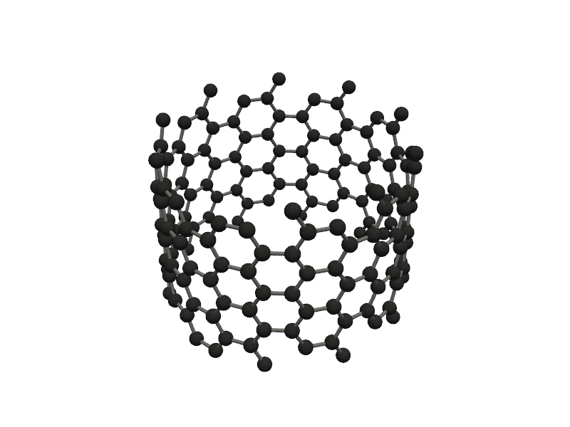
from PyGamLab.structures.GAM_architectures import Nanotube_Generator
nanotube = Nanotube_Generator(n=10, m=10, length=10.0, atom_type='C')
nanotube_atoms = nanotube.get_atoms()
Molecular_Visualizer(nanotube_atoms, format='pyvista')

Visualizing 160 atoms using pyvista format...

/Users/apm/anaconda3/envs/DL/lib/python3.10/site-packages/pyvista/jupyter/notebook.py:56: UserWarning:

Failed to use notebook backend:

No module named 'trame'

Falling back to a static output.

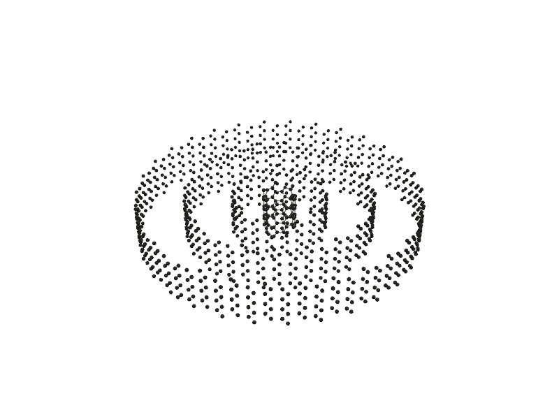
#lets go for more advanced nano tubes
nanotube = Nanotube_Generator(n=5, m=5, length=10.0, atom_type='C', multi_wall=[(10,10), (20, 20), (30,30)])
nanotube_atoms = nanotube.get_atoms()
Molecular_Visualizer(nanotube_atoms, format='pyvista')

Visualizing 1040 atoms using pyvista format...

/Users/apm/anaconda3/envs/DL/lib/python3.10/site-packages/pyvista/jupyter/notebook.py:56: UserWarning:

Failed to use notebook backend:

No module named 'trame'

Falling back to a static output.

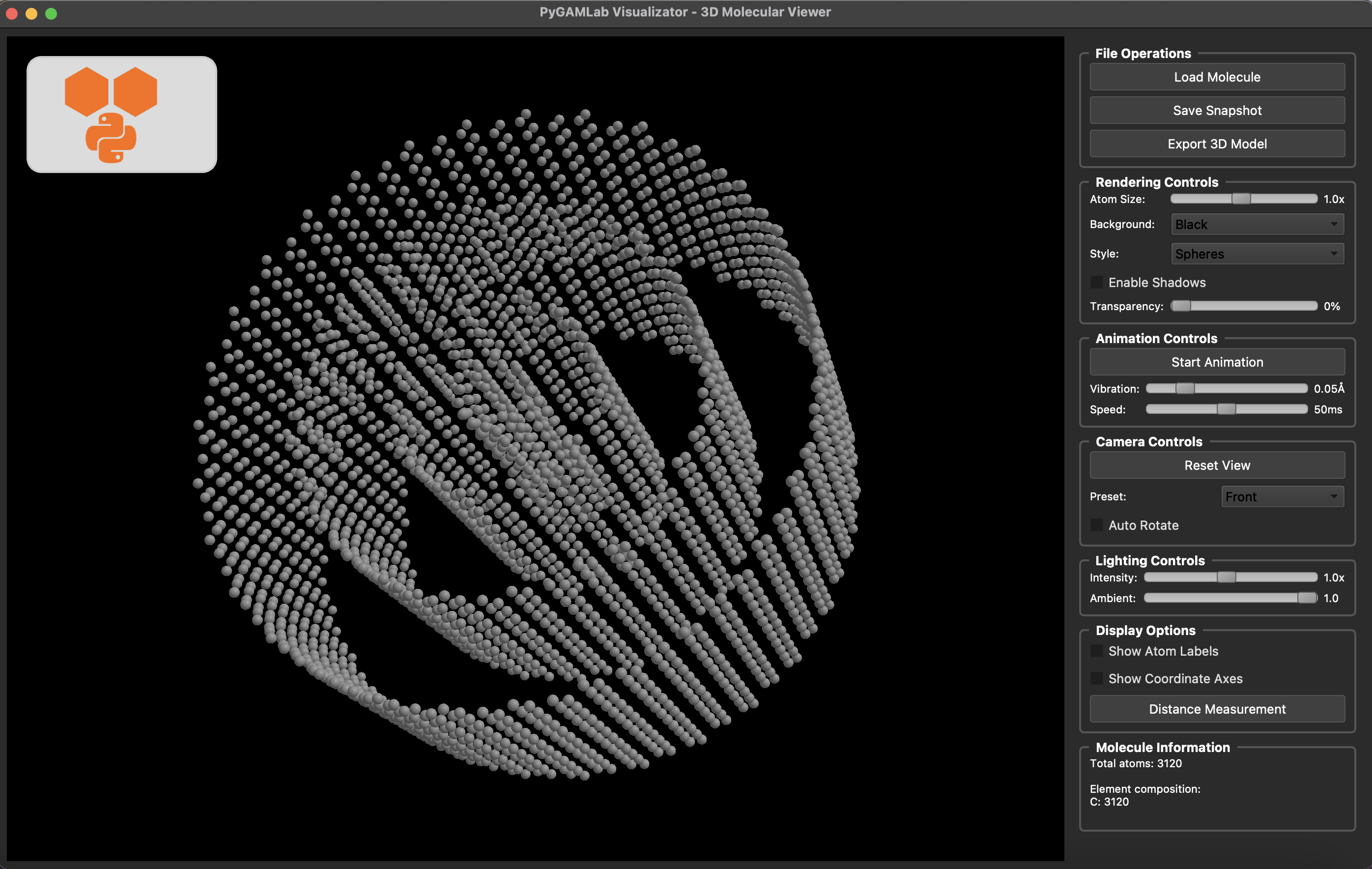
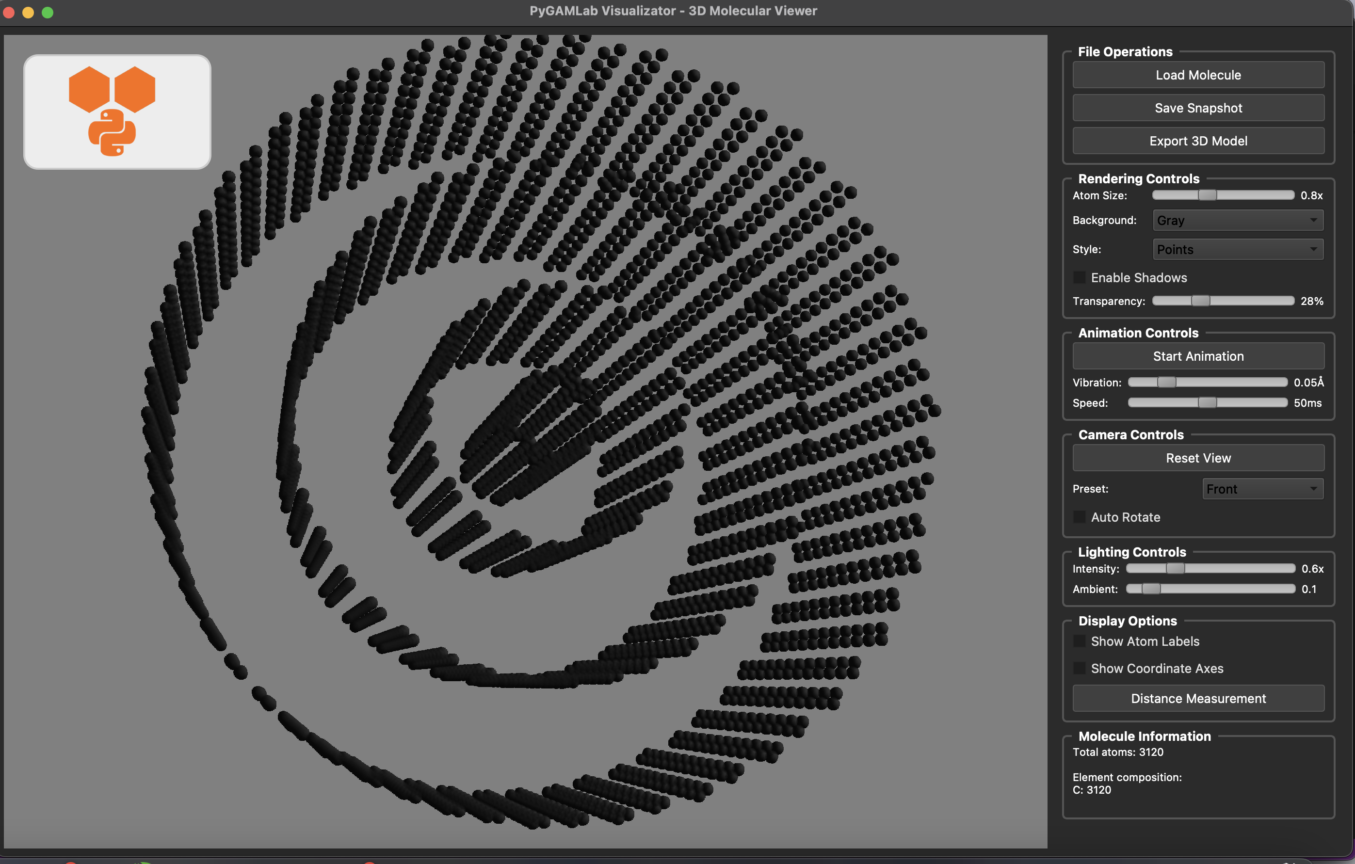
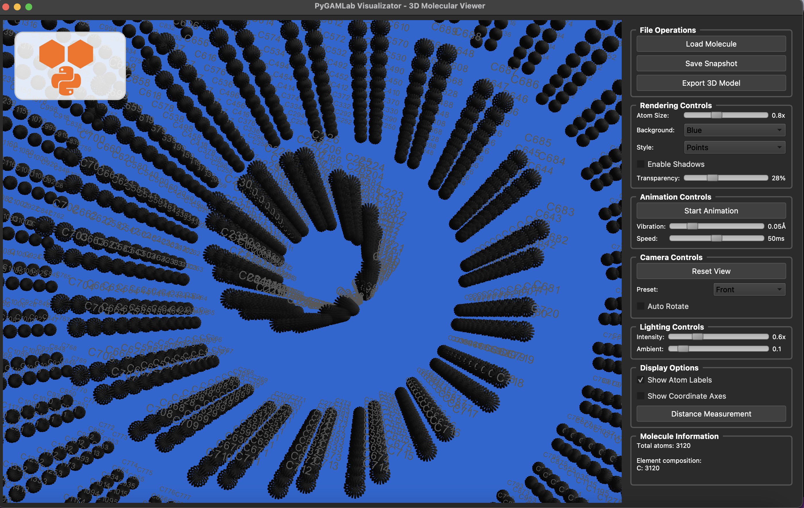
#Also you can use Gamvis which is based on VTK for visualization
nanotube = Nanotube_Generator(n=5, m=5, length=30.0, atom_type='C', multi_wall=[(10,10), (20, 20), (30,30)])
nanotube_atoms = nanotube.get_atoms()
#just you need to change format to 'gamvis'
Molecular_Visualizer(nanotube_atoms, format='gamvis')

Visualizing 3120 atoms using gamvis format...
=== PyGAMLab Visualizator Debug Info ===
Python version: 3.10.13 | packaged by conda-forge | (main, Dec 23 2023, 15:35:25) [Clang 16.0.6 ]
PyQt5 version: 5.15.2
Platform: Darwin 24.3.0
Creating main window...
Loading 3120 atoms...

QPixmap::scaled: Pixmap is a null pixmap
qt.qpa.window: <QNSWindow: 0x3980feb20; contentView=<QNSView: 0x39559f020; QCocoaWindow(0x3955a5770, window=QWidgetWindow(0x395572f40, name="QWidgetClassWindow"))>> has active key-value observers (KVO)! These will stop working now that the window is recreated, and will result in exceptions when the observers are removed. Break in QCocoaWindow::recreateWindowIfNeeded to debug.

Showing window...
Initializing VTK interactor...
Application ready!

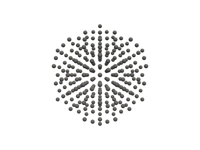
from PyGamLab.structures.GAM_architectures import Nanoparticle_Generator
npg = Nanoparticle_Generator(element="Au", size_nm=2.0)
npg_atoms = npg.get_atoms()
Molecular_Visualizer(npg_atoms, format='pyvista')

Visualizing 249 atoms using pyvista format...

/Users/apm/anaconda3/envs/DL/lib/python3.10/site-packages/pyvista/jupyter/notebook.py:56: UserWarning:

Failed to use notebook backend:

No module named 'trame'

Falling back to a static output.

More examples are available in …..

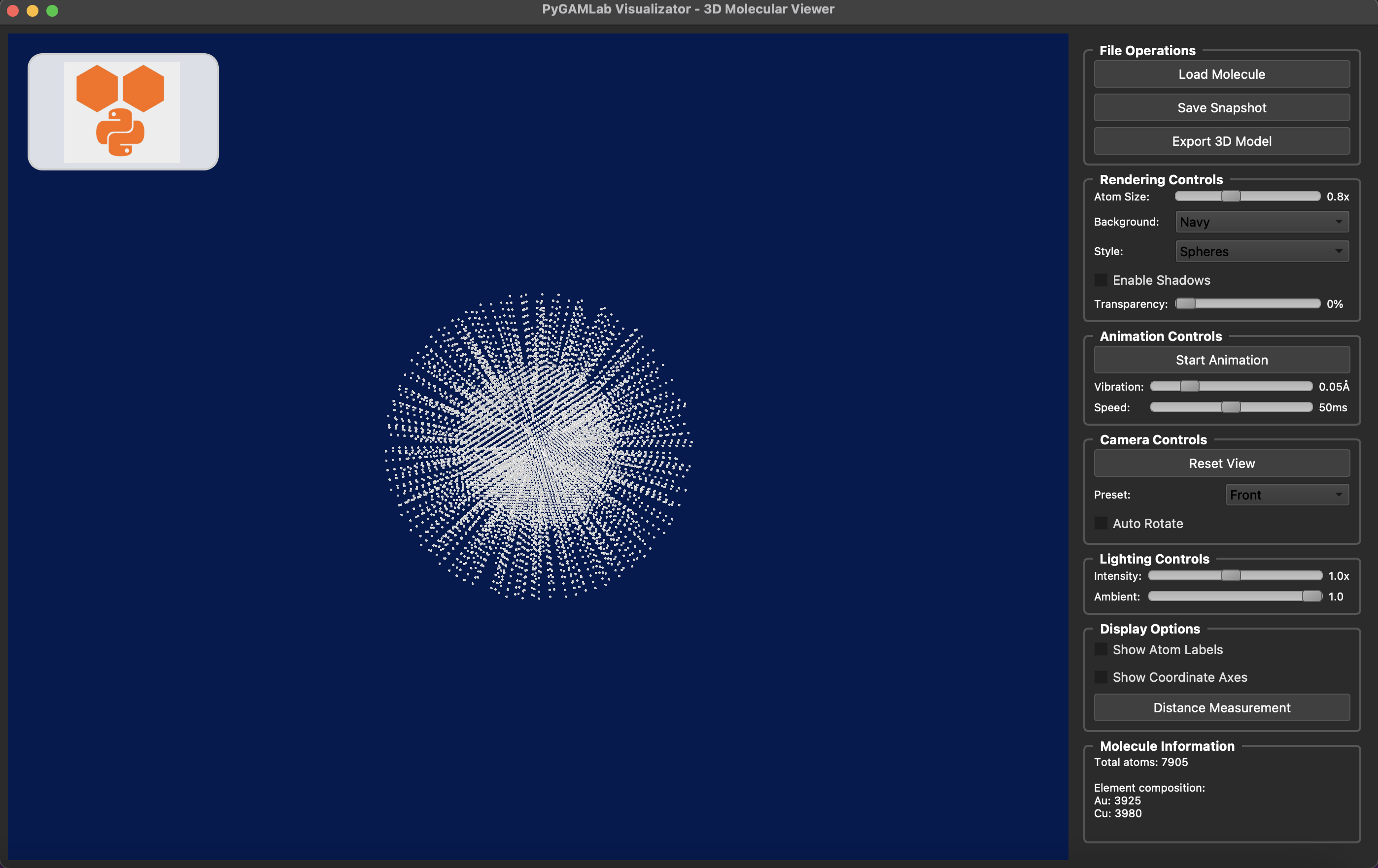
from PyGamLab.structures.GAM_architectures import Nanoparticle_Generator
npg = Nanoparticle_Generator(element="Au", size_nm=5.0, coating=("Cu", 2.0))
npg_atoms = npg.get_atoms()
Molecular_Visualizer(npg_atoms, format='gamvis')

Visualizing 7905 atoms using gamvis format...
=== PyGAMLab Visualizator Debug Info ===
Python version: 3.10.13 | packaged by conda-forge | (main, Dec 23 2023, 15:35:25) [Clang 16.0.6 ]
PyQt5 version: 5.15.2
Platform: Darwin 24.3.0
Creating main window...
Loading 7905 atoms...

QPixmap::scaled: Pixmap is a null pixmap
qt.qpa.window: <QNSWindow: 0x37e5ddd60; contentView=<QNSView: 0x3bdb09bd0; QCocoaWindow(0x37e5a3660, window=QWidgetWindow(0x37e5ae740, name="QWidgetClassWindow"))>> has active key-value observers (KVO)! These will stop working now that the window is recreated, and will result in exceptions when the observers are removed. Break in QCocoaWindow::recreateWindowIfNeeded to debug.

Showing window...
Initializing VTK interactor...
Application ready!

5. Databases¶

One of the most essential needs of researchers and engineers in materials science is access to reliable databases. Whether you’re studying crystal structures, mechanical properties, or electronic characteristics, having a unified way to query and retrieve data saves enormous time and effort.

In the scientific world, data is everything — from experimental measurements to computational predictions — and these data are often stored in distributed databases across different platforms.

However, accessing them is not always straightforward: some provide web interfaces, others require REST APIs, and many use unique data structures or access protocols.

The PyGamLab Databases module was designed to make this process simpler, unified, and accessible from a single platform.

Why Access to Databases Matters¶

Researchers need databases for a variety of reasons:

Designing new materials using reference data (like lattice parameters, space groups, or electronic band structures).
Verifying experimental results by comparing them to reported literature or simulation data.
Training AI or ML models for property prediction or material discovery.
Generating structure prototypes for simulation inputs.
Performing high-throughput screening for materials with target properties (e.g., low bandgap, high conductivity, etc.).

Without a common platform, scientists often have to juggle between multiple APIs, formats, and authentication systems.

PyGamLab’s databases module solves this problem by providing a single, unified API that communicates with multiple popular databases.

Supported Databases¶

Currently, the PyGamLab Databases module integrates access to several major material databases:

Crystallography Open Database (COD) –

An open-source collection of crystal structures, ideal for retrieving atomic coordinates, space groups, and unit cell parameters for inorganic and organic compounds.
AFLOW (Automatic Flow for Materials Discovery) –

A computational database providing mechanical, thermal, and electronic properties of materials obtained from high-throughput ab initio calculations.
Materials Project –

One of the most widely used materials databases, offering band structures, formation energies, elastic tensors, and symmetry information for thousands of compounds.
JARVIS (NIST) –

A comprehensive materials database developed by NIST, which includes quantum mechanical, machine learning, and experimental data across a wide range of materials.

The Challenge of Using Multiple Databases¶

Each of these databases comes with its own access method:

Some are available only through web-based graphical interfaces (GUIs), where users manually search for materials and download data.
Others provide Python wrappers, which require separate installation and different query syntax.
Many support RESTful APIs, which require constructing HTTP requests, managing endpoints, and handling JSON responses — often with slightly different structures.

This diversity makes it hard to combine data across databases or perform automated, large-scale analyses.

PyGamLab’s Unified Solution: `Explorer`¶

To address this problem, PyGamLab introduces the ``Explorer`` class within the Databases module — a unified interface that connects you to multiple data sources using a consistent syntax and logic.

With the Explorer, you can: - Retrieve data from multiple sources
(COD, AFLOW, Materials Project, JARVIS).
- Query specific materials, compositions, or properties.
- Synchronize data between sources for cross-validation.
- Extract structured results ready for analysis or machine learning
workflows.

You don’t need to worry about endpoints, tokens, or inconsistent formats — PyGamLab handles the communication and returns clean, standardized data objects that can be directly used in your workflow.

Advantages of the Databases Module¶

Unified Access – One consistent interface for multiple databases.
Cross-Database Synchronization – Retrieve and compare data from several sources at once.
Automation Ready – Integrate directly into your data pipelines or AI workflows.
Standardized Output – No more inconsistent formats or API confusion.
Extensible – New databases can be easily added in future versions.

Example Usage¶

#you can fetch data from AFLOW

from PyGamLab.databases import Aflow_Explorer
my_explorer=Aflow_Explorer()

my_explorer.search_materials(formula="Cs1F3Mg1", max_results=3,batch_size=10)

[{'auid': 'aflow:141bd22d5b219f1f',
  'prototype': 'Cs1F3Mg1_ICSD_290359',
  'spacegroup_relax': 221,
  'dft_type': ['PAW_PBE'],
  'spinD': array([0, 0, 0, 0, 0]),
  'spinF': 0,
  'enthalpy_formation_cell': -15.9531,
  'natoms': 5},
 {'auid': 'aflow:494166da0e7a6134',
  'prototype': 'Cs1F3Mg1_ICSD_49584',
  'spacegroup_relax': 221,
  'dft_type': ['PAW_PBE'],
  'spinD': array([0, 0, 0, 0, 0]),
  'spinF': 0,
  'enthalpy_formation_cell': -15.9536,
  'natoms': 5},
 {'auid': 'aflow:4c5ca27e65d9772c',
  'prototype': 'T0009.CAB',
  'spacegroup_relax': 221,
  'dft_type': ['PAW_PBE'],
  'spinD': array([0, 0, 0, 0, 0]),
  'spinF': 0,
  'enthalpy_formation_cell': -6.56372,
  'natoms': 5}]

#so now you have different aflow id and also you can specify which one you want to get their properties
#you can get electrical porperty, mechanical and .....

#for instance auid of 'aflow:141bd22d5b219f1f' is ok
electronic_data=my_explorer.fetch_electronic_properties(auid='aflow:141bd22d5b219f1f')

print(electronic_data)

{'formula': 'Cs1F3Mg1', 'bandgap': 6.721, 'bandgap_fit': 9.97291, 'bandgap_type': 'insulator-direct', 'delta_elec_energy_convergence': 1.2486e-05, 'delta_elec_energy_threshold': 0.0001, 'ldau_TLUJ': None, 'dft_type': ['PAW_PBE'], 'bader_atomic_volumes': array([27.44  , 14.2738, 14.2738, 14.2745,  6.4306]), 'bader_net_charges': array([ 0.9138, -0.8733, -0.8733, -0.8734,  1.7062]), 'spinD': array([0, 0, 0, 0, 0]), 'spinF': 0, 'spin_atom': 0, 'spin_cell': 0, 'scintillation_attenuation_length': 2.4419}

#also you can get mechanical properties
mechanical_data=my_explorer.fetch_mechanical_properties(auid='aflow:141bd22d5b219f1f')
print(mechanical_data)

{'formula': 'Cs1F3Mg1', 'bulk_modulus_reuss': None, 'bulk_modulus_voigt': None, 'bulk_modulus_vrh': None, 'shear_modulus_reuss': None, 'shear_modulus_voigt': None, 'shear_modulus_vrh': None, 'poisson_ratio': None, 'elastic_anisotropy': None, 'stress_tensor': array([ 0.97,  0.  , -0.  ,  0.  ,  0.97,  0.  , -0.  ,  0.  ,  0.97]), 'forces': array([[ 0.,  0.,  0.],
       [-0.,  0.,  0.],
       [ 0.,  0.,  0.],
       [ 0.,  0., -0.],
       [ 0.,  0.,  0.]]), 'Pulay_stress': 0, 'pressure': 0, 'pressure_residual': 0.97}

#you can also get thermodynamic properties
thermodynamic_data=my_explorer.fetch_thermodynamic_properties(auid='aflow:141bd22d5b219f1f')
print(thermodynamic_data)

{'formula': 'Cs1F3Mg1', 'acoustic_debye': None, 'debye': None, 'gruneisen': None, 'heat_capacity_Cp_300K': None, 'heat_capacity_Cv_300K': None, 'thermal_conductivity_300K': None, 'thermal_expansion_300K': None, 'bulk_modulus_isothermal_300K': None, 'bulk_modulus_static_300K': None, 'entropy_atom': 0.00118258, 'entropy_cell': 0.00591288, 'enthalpy_atom': -4.79552, 'enthalpy_cell': -23.9776, 'enthalpy_formation_atom': -3.19062, 'enthalpy_formation_cell': -15.9531, 'energy_atom': -4.79552, 'energy_cell': -23.9776, 'energy_cutoff': array([560]), 'entropic_temperature': 38963.2}

#also you can get structure

structure_data=my_explorer.fetch_structure(auid='aflow:141bd22d5b219f1f')
print(structure_data)

{'formula': 'Cs1F3Mg1', 'Bravais_lattice_orig': 'CUB', 'Bravais_lattice_relax': 'CUB', 'Pearson_symbol_orig': 'cP5', 'Pearson_symbol_relax': 'cP5', 'lattice_system_orig': 'cubic', 'lattice_system_relax': 'cubic', 'lattice_variation_orig': 'CUB', 'lattice_variation_relax': 'CUB', 'spacegroup_orig': 221, 'spacegroup_relax': 221, 'sg': ['Pm-3m #221', 'Pm-3m #221', 'Pm-3m #221'], 'sg2': ['Pm-3m #221', 'Pm-3m #221', 'Pm-3m #221'], 'prototype': 'Cs1F3Mg1_ICSD_290359', 'stoich': [0.2, 0.6, 0.2], 'stoichiometry': array([0.2, 0.6, 0.2]), 'geometry': array([ 4.2486519,  4.2486519,  4.2486519, 90.       , 90.       ,
       90.       ]), 'natoms': 5, 'nspecies': 3, 'nbondxx': array([4.2487, 3.0043, 3.6794, 3.0043, 2.1243, 4.2487]), 'composition': array([1, 3, 1]), 'compound': 'Cs1F3Mg1', 'species': ['Cs', 'F', 'Mg'], 'species_pp': ['Cs_sv', 'F', 'Mg_pv'], 'species_pp_ZVAL': array([9, 7, 8]), 'species_pp_version': ['Cs_sv:PAW_PBE:08Apr2002', 'F:PAW_PBE:08Apr2002', 'Mg_pv:PAW_PBE:06Sep2000'], 'positions_cartesian': array([[0.     , 0.     , 0.     ],
       [2.12433, 2.12433, 0.     ],
       [0.     , 2.12433, 2.12433],
       [2.12433, 0.     , 2.12433],
       [2.12433, 2.12433, 2.12433]]), 'positions_fractional': array([[0. , 0. , 0. ],
       [0.5, 0.5, 0. ],
       [0. , 0.5, 0.5],
       [0.5, 0. , 0.5],
       [0.5, 0.5, 0.5]]), 'valence_cell_iupac': 6, 'valence_cell_std': 24, 'volume_atom': 15.3385, 'volume_cell': 76.6926, 'density': 4.63796}

#also for more efficient you can get all properties at once
all_data=my_explorer.fetch_all_data(auid='aflow:141bd22d5b219f1f')
print(all_data)

{'electronic_prop': {'formula': 'Cs1F3Mg1', 'bandgap': 6.721, 'bandgap_fit': 9.97291, 'bandgap_type': 'insulator-direct', 'delta_elec_energy_convergence': 1.2486e-05, 'delta_elec_energy_threshold': 0.0001, 'ldau_TLUJ': None, 'dft_type': ['PAW_PBE'], 'bader_atomic_volumes': array([27.44  , 14.2738, 14.2738, 14.2745,  6.4306]), 'bader_net_charges': array([ 0.9138, -0.8733, -0.8733, -0.8734,  1.7062]), 'spinD': array([0, 0, 0, 0, 0]), 'spinF': 0, 'spin_atom': 0, 'spin_cell': 0, 'scintillation_attenuation_length': 2.4419}, 'mechanical_prop': {'formula': 'Cs1F3Mg1', 'bulk_modulus_reuss': None, 'bulk_modulus_voigt': None, 'bulk_modulus_vrh': None, 'shear_modulus_reuss': None, 'shear_modulus_voigt': None, 'shear_modulus_vrh': None, 'poisson_ratio': None, 'elastic_anisotropy': None, 'stress_tensor': array([ 0.97,  0.  , -0.  ,  0.  ,  0.97,  0.  , -0.  ,  0.  ,  0.97]), 'forces': array([[ 0.,  0.,  0.],
       [-0.,  0.,  0.],
       [ 0.,  0.,  0.],
       [ 0.,  0., -0.],
       [ 0.,  0.,  0.]]), 'Pulay_stress': 0, 'pressure': 0, 'pressure_residual': 0.97}, 'thermo_prop': {'formula': 'Cs1F3Mg1', 'acoustic_debye': None, 'debye': None, 'gruneisen': None, 'heat_capacity_Cp_300K': None, 'heat_capacity_Cv_300K': None, 'thermal_conductivity_300K': None, 'thermal_expansion_300K': None, 'bulk_modulus_isothermal_300K': None, 'bulk_modulus_static_300K': None, 'entropy_atom': 0.00118258, 'entropy_cell': 0.00591288, 'enthalpy_atom': -4.79552, 'enthalpy_cell': -23.9776, 'enthalpy_formation_atom': -3.19062, 'enthalpy_formation_cell': -15.9531, 'energy_atom': -4.79552, 'energy_cell': -23.9776, 'energy_cutoff': array([560]), 'entropic_temperature': 38963.2}, 'structure': {'formula': 'Cs1F3Mg1', 'Bravais_lattice_orig': 'CUB', 'Bravais_lattice_relax': 'CUB', 'Pearson_symbol_orig': 'cP5', 'Pearson_symbol_relax': 'cP5', 'lattice_system_orig': 'cubic', 'lattice_system_relax': 'cubic', 'lattice_variation_orig': 'CUB', 'lattice_variation_relax': 'CUB', 'spacegroup_orig': 221, 'spacegroup_relax': 221, 'sg': ['Pm-3m #221', 'Pm-3m #221', 'Pm-3m #221'], 'sg2': ['Pm-3m #221', 'Pm-3m #221', 'Pm-3m #221'], 'prototype': 'Cs1F3Mg1_ICSD_290359', 'stoich': [0.2, 0.6, 0.2], 'stoichiometry': array([0.2, 0.6, 0.2]), 'geometry': array([ 4.2486519,  4.2486519,  4.2486519, 90.       , 90.       ,
       90.       ]), 'natoms': 5, 'nspecies': 3, 'nbondxx': array([4.2487, 3.0043, 3.6794, 3.0043, 2.1243, 4.2487]), 'composition': array([1, 3, 1]), 'compound': 'Cs1F3Mg1', 'species': ['Cs', 'F', 'Mg'], 'species_pp': ['Cs_sv', 'F', 'Mg_pv'], 'species_pp_ZVAL': array([9, 7, 8]), 'species_pp_version': ['Cs_sv:PAW_PBE:08Apr2002', 'F:PAW_PBE:08Apr2002', 'Mg_pv:PAW_PBE:06Sep2000'], 'positions_cartesian': array([[0.     , 0.     , 0.     ],
       [2.12433, 2.12433, 0.     ],
       [0.     , 2.12433, 2.12433],
       [2.12433, 0.     , 2.12433],
       [2.12433, 2.12433, 2.12433]]), 'positions_fractional': array([[0. , 0. , 0. ],
       [0.5, 0.5, 0. ],
       [0. , 0.5, 0.5],
       [0.5, 0. , 0.5],
       [0.5, 0.5, 0.5]]), 'valence_cell_iupac': 6, 'valence_cell_std': 24, 'volume_atom': 15.3385, 'volume_cell': 76.6926, 'density': 4.63796}, 'meta_data': {}}

#so you can also go for using other databases like Materials Porjct, Jarvis, COD
#just you can create different explorer but teh methods are similar

#for COD -->
from PyGamLab.databases import COD_Explorer
my_explorer_cod=COD_Explorer()


#for Jarviis -->

from PyGamLab.databases import Jarvis_Explorer

my_jarvis_explorer=Jarvis_Explorer()


#for Materials Project -->
from PyGamLab.databases import MaterialsProject_Explorer
#just note that for Materials Project you need to have an api key from their website
#you can sign up and get your api key and put it here
#website : https://next-gen.materialsproject.org/api
my_explorer_mp=MaterialsProject_Explorer(api_key="your_api_key_here")



#then on you robject you can use similar methods like search_materials, fetch_electronic_properties and .....

Also Gamlab provide more efficient way for fetching data from databases You can use GAM_Explorer which can connect to different databases at once and is wrapper for different explorers and you can call them with specifying backend

from PyGamLab.databases import GAM_Explorer
gam_explorer=GAM_Explorer(backend='your backend here like aflow, jarvis, mp, cod')

you can specify backend there and for instance backend=‘aflow’ or backend=‘jarvis’ or backend=‘mp’ or backend=‘cod’ and it turn to Aflow_Explorer, Jarvis_Explorer, MaterialsProject_Explorer, COD_Explorer respectively and then you can use similar methods like search_materials, fetch_electronic_properties and

and then you can see from which database the data is fetched

6. Data Analysis¶

In every area of scientific research, one thing is always constant — data.

Researchers spend a significant part of their time collecting, analyzing, and interpreting experimental or simulation data to extract meaningful insights.

Whether you are in a materials science laboratory, performing nanostructure experiments, or running computational simulations, your work often produces raw data — sometimes clean and structured, but often noisy, incomplete, or only presented in graphical form by instrument software.

Extracting usable information from such data requires significant effort — converting, processing, plotting, and calculating derived parameters.

To simplify this process, PyGamLab introduces the ``data_analysis`` module — a powerful collection of tools designed to help researchers load, analyze, and visualize their data with minimal effort.

Why PyGamLab’s Data Analysis Module?¶

In experimental and computational materials science, researchers often face challenges such as:

Instrument software outputting only images instead of numeric data.
Inconsistent data formats (CSV, TXT, Excel, etc.).
The need for custom analysis functions for each type of experiment.
Manual plotting and data cleaning steps repeated for every dataset.

The ``data_analysis`` module solves these challenges by providing a unified framework for working with your laboratory or simulation data directly in Python.

It allows you to load raw data, analyze it using specialized functions, plot results, and extract meaningful parameters — all in one place.

Core Design Philosophy¶

Each function in the data_analysis module is designed to correspond to a specific experimental technique or characterization tool.

For example, one function might process XRD (X-ray diffraction) data, while another might analyze Raman spectra, UV-Vis, SEM image data, or mechanical stress-strain results.

The philosophy is simple: > You focus on your science, and PyGamLab takes care of the data handling and analysis logic.

How It Works¶

Most functions in this module share a common interface for simplicity and consistency.

Here’s how a typical data analysis workflow looks:

Prepare your data

Your data should be in a ``pandas.DataFrame`` format, where each column represents a measured variable (for example: wavelength, intensity, time, voltage, etc.).
Choose your analysis function

Each experimental method (e.g., XRD, Raman, IV, TEM, etc.) has its own specialized function within the data_analysis module.
Specify the application type

Most functions accept an argument called application, which determines what action you want to perform.

Common options include:
- "plot" → visualize your data in different styles (line, scatter, log-scale, etc.)
- "calculate" → compute quantitative results (like peak positions, intensity ratios, etc.)
- "process" → perform background removal, smoothing, normalization, or advanced signal processing
Run and interpret results

The output can be a plot, processed data, or calculated numerical results ready for publication or further computation.

Example: Analyzing NMR Data¶

#first of all you must import pandas
import pandas as pd

#pd has two function one is read_csv to read csv files and another read_excel to read excel files
#to read csv files
data_csv=pd.read_csv('your_file_name.csv')
#to read excel files
data_excel=pd.read_excel('your_file_name.xlsx')


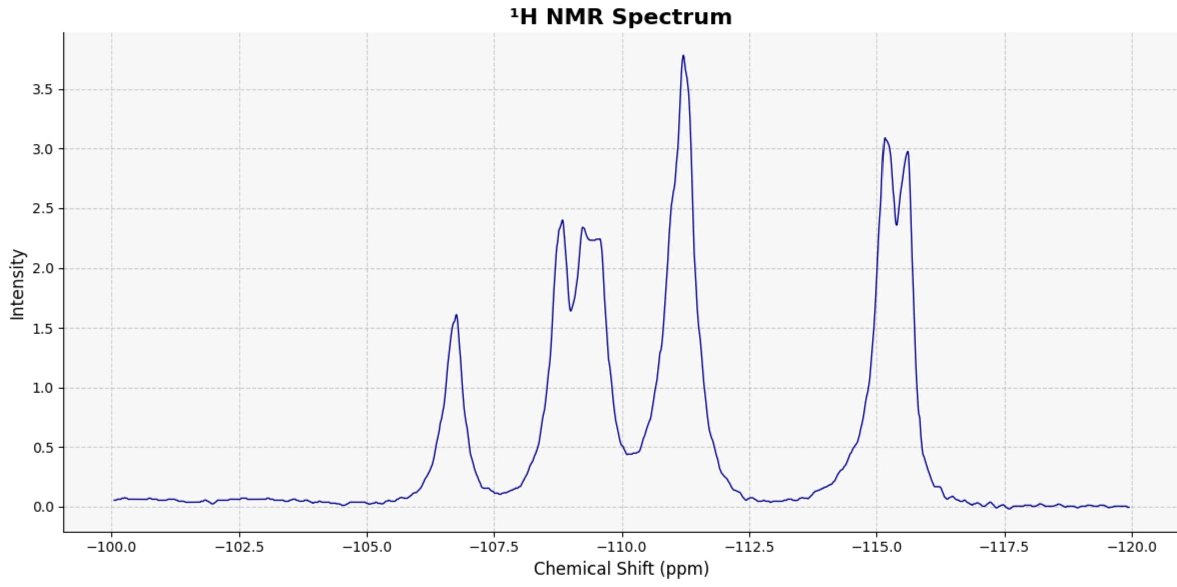
from PyGamLab.Data_Analysis import NMR_Analysis

#this function get data as dataframe and application parameter
#application parameter means which type of analysis you want to do

#for instance plotting

NMR_Analysis(data=data_csv, application='plot')

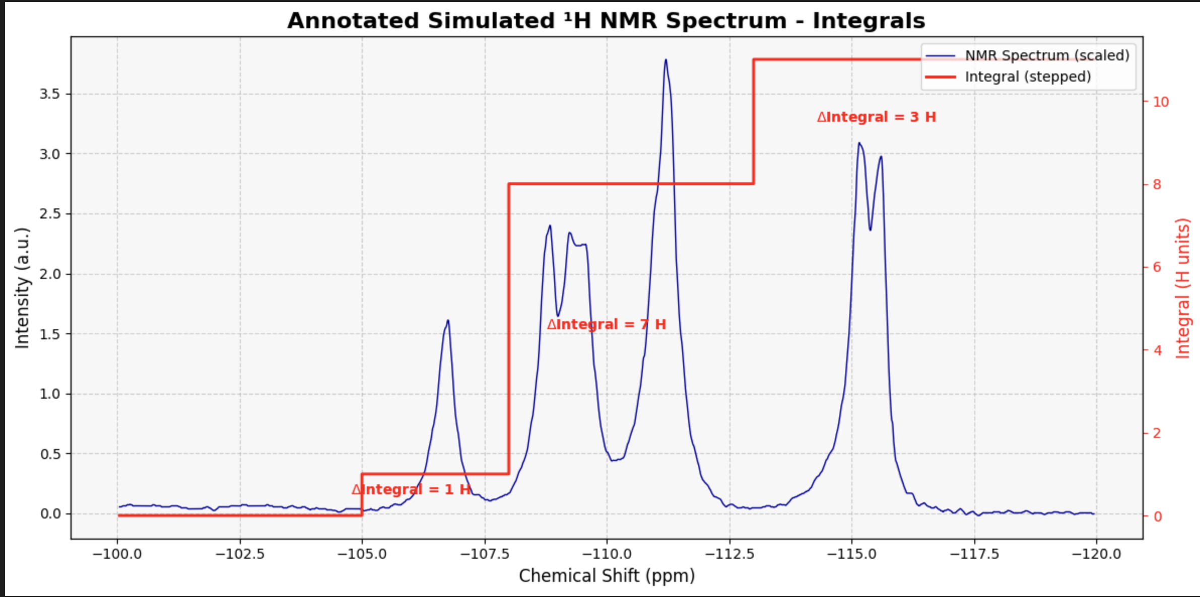
my_peak_regions = {
    'Aromatic': (-107, -105),
    'Benzylic CH₂': (-112, -108),
    'Acetyl CH₃': (-118, -113)
}

# Call the function to generate the plot with integral steps
NMR_Analysis(data, application='plot_with_integrals', peak_regions=my_peak_regions)

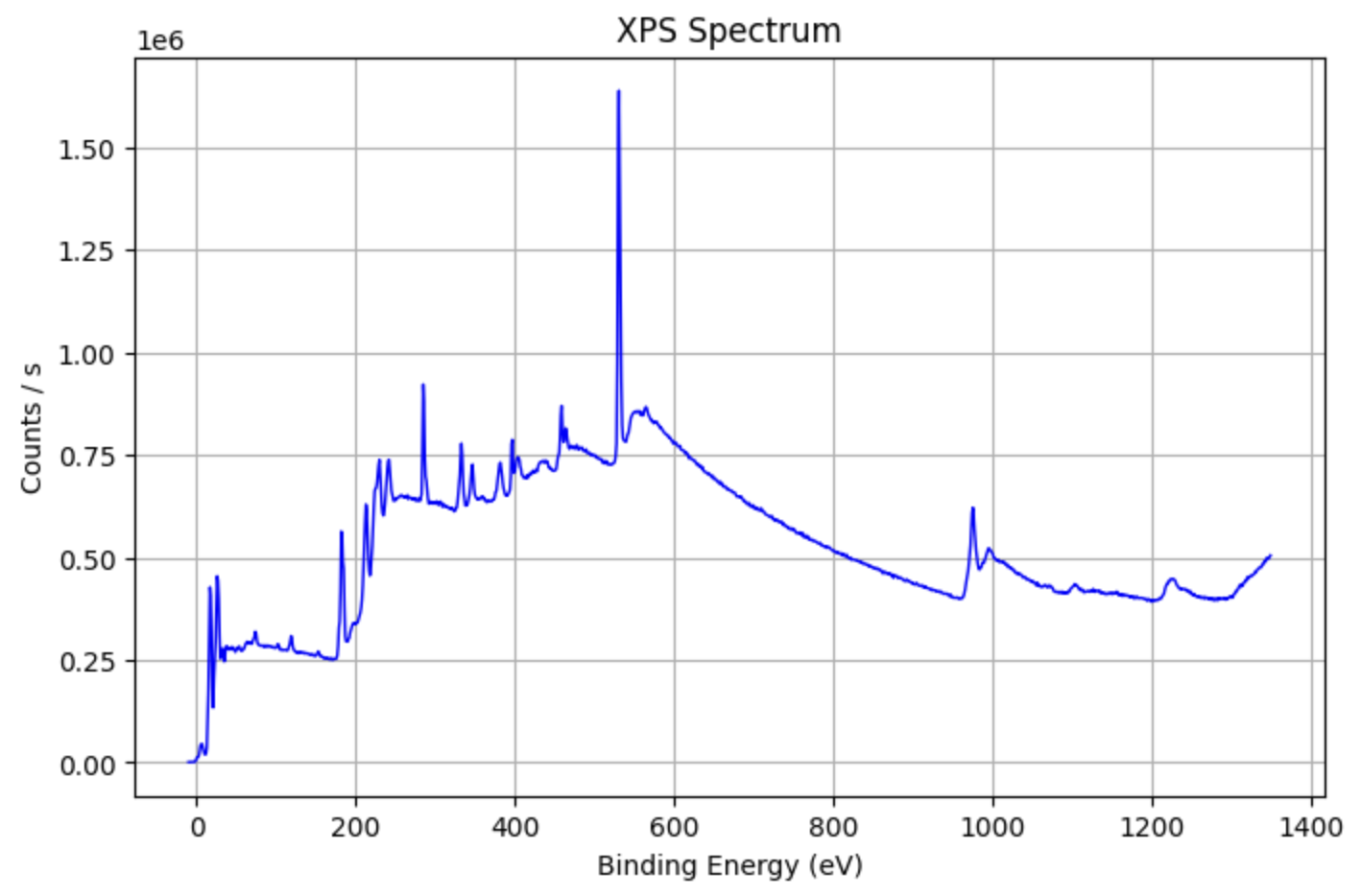
Example: Analyzing XPS Data¶

XPS_data=pd.read_excel('your_file_name.xlsx')
from PyGamLab.Data_Analysis import XPS_Analysis

XPS_Analysis(data=XPS_data, application='plot')

peaks = XPS_Analysis(df, application='peak_detection', peak_prominence=10000)
for p in peaks:
    print(f"Peak at {p['energy']:.2f} eV, height {p['counts']:.1f}, FWHM {p['width']:.2f} points")

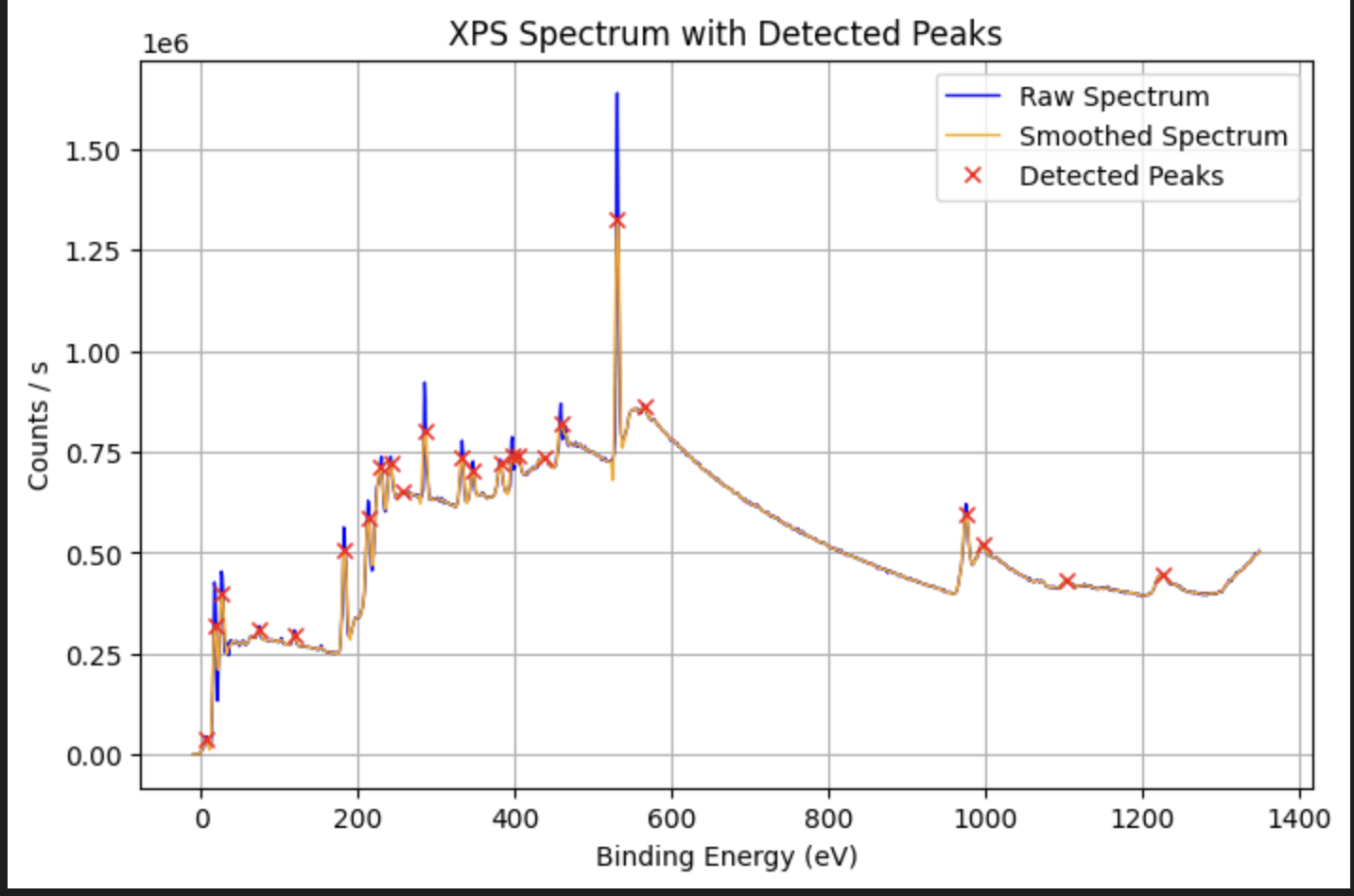
#Peak at 1227.08 eV, height 447819.0, FWHM 23.11 points
#Peak at 1105.08 eV, height 433361.0, FWHM 10.59 points
#Peak at 997.08 eV, height 517901.0, FWHM 13.04 points
#Peak at 976.08 eV, height 621396.0, FWHM 9.79 points
#Peak at 565.08 eV, height 867297.0, FWHM 42.23 points
#Peak at 531.08 eV, height 1638660.0, FWHM 8.20 points
#Peak at 460.08 eV, height 815931.0, FWHM 42.35 points
#Peak at 438.08 eV, height 731991.0, FWHM 13.62 points
#Peak at 404.08 eV, height 745177.0, FWHM 12.58 points
#Peak at 398.08 eV, height 728148.0, FWHM 3.80 points
#Peak at 382.08 eV, height 731348.0, FWHM 7.37 points
#Peak at 347.08 eV, height 726994.0, FWHM 6.32 points
#Peak at 333.08 eV, height 778125.0, FWHM 6.33 points
#Peak at 286.08 eV, height 879292.0, FWHM 6.50 points
#Peak at 257.08 eV, height 651998.0, FWHM 16.93 points
#Peak at 242.08 eV, height 738299.0, FWHM 6.83 points
#Peak at 229.08 eV, height 725264.0, FWHM 7.39 points
#Peak at 213.08 eV, height 629412.0, FWHM 5.06 points
#Peak at 183.08 eV, height 559701.0, FWHM 6.10 points
#Peak at 119.08 eV, height 308560.0, FWHM 5.81 points
#Peak at 74.08 eV, height 319002.0, FWHM 37.19 points
#Peak at 26.08 eV, height 454384.0, FWHM 5.36 points
#Peak at 18.08 eV, height 406393.0, FWHM 4.21 points
#Peak at 7.08 eV, height 45308.4, FWHM 5.49 points

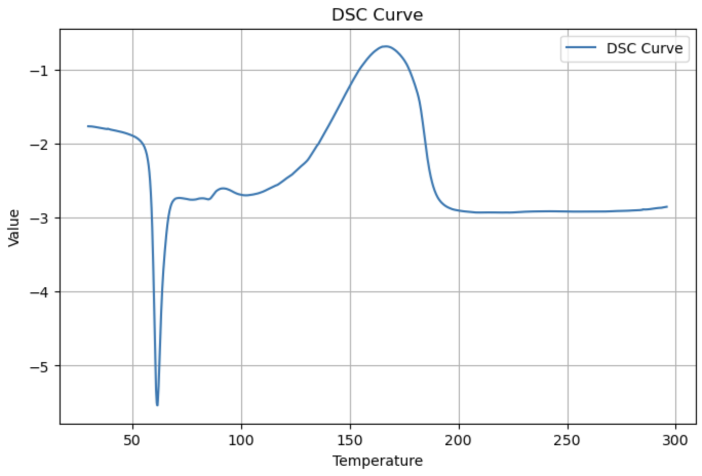
DSC¶

from PyGamLab.Data_Analysis import DSC

dsc_data=pd.read_excel('your_file_name.xlsx')

DSC(data=dsc_data, application='plot')

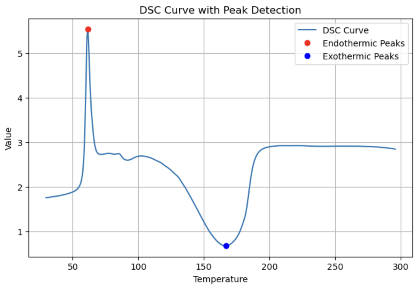
peaks = DSC(dsc_data, application="peak_detection", prominence=2.0, distance=10)

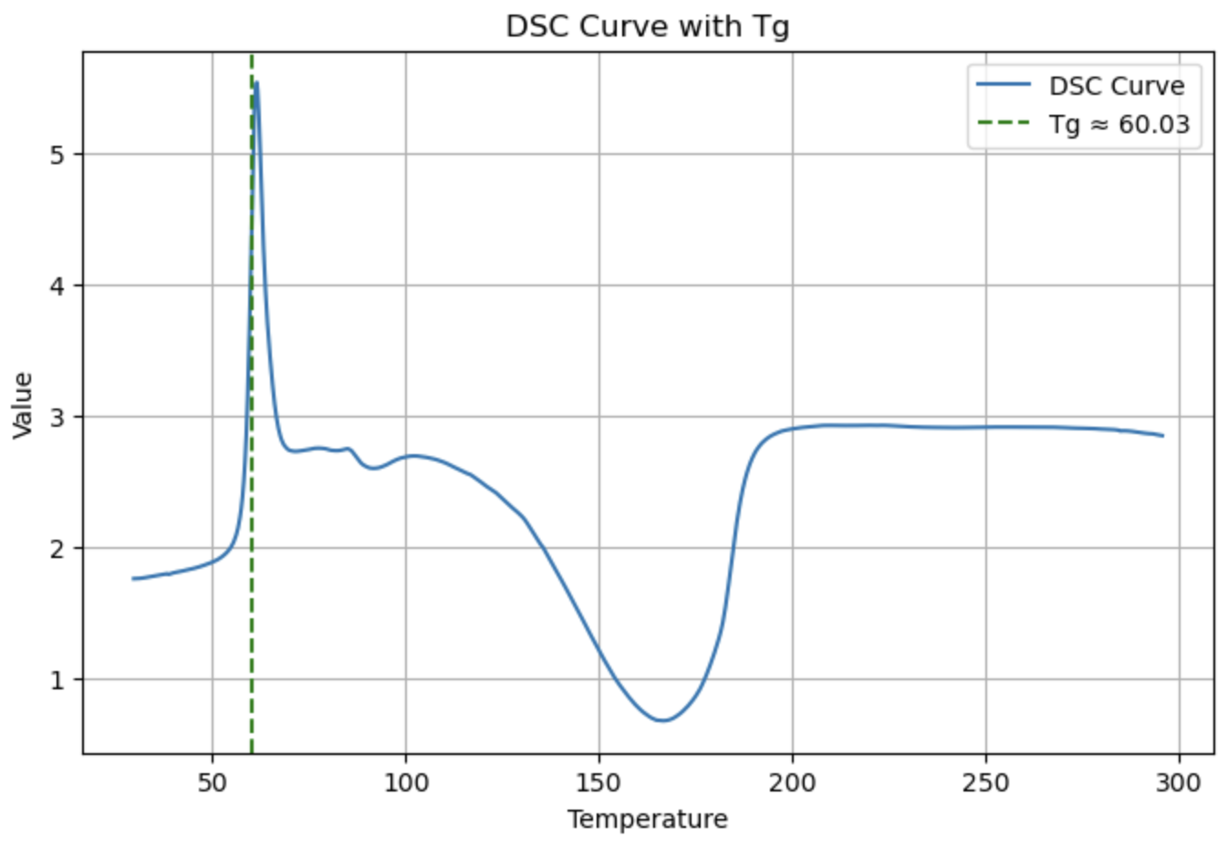
DSC(dsc_data, application="Tg")

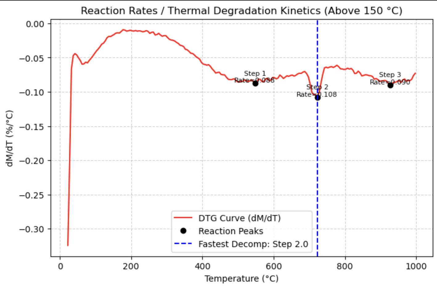
TGA¶

from PyGamLab.Data_Analysis import TGA

data=pd.read_excel('your_file_name.xlsx')
TGA(data, application="peaks")

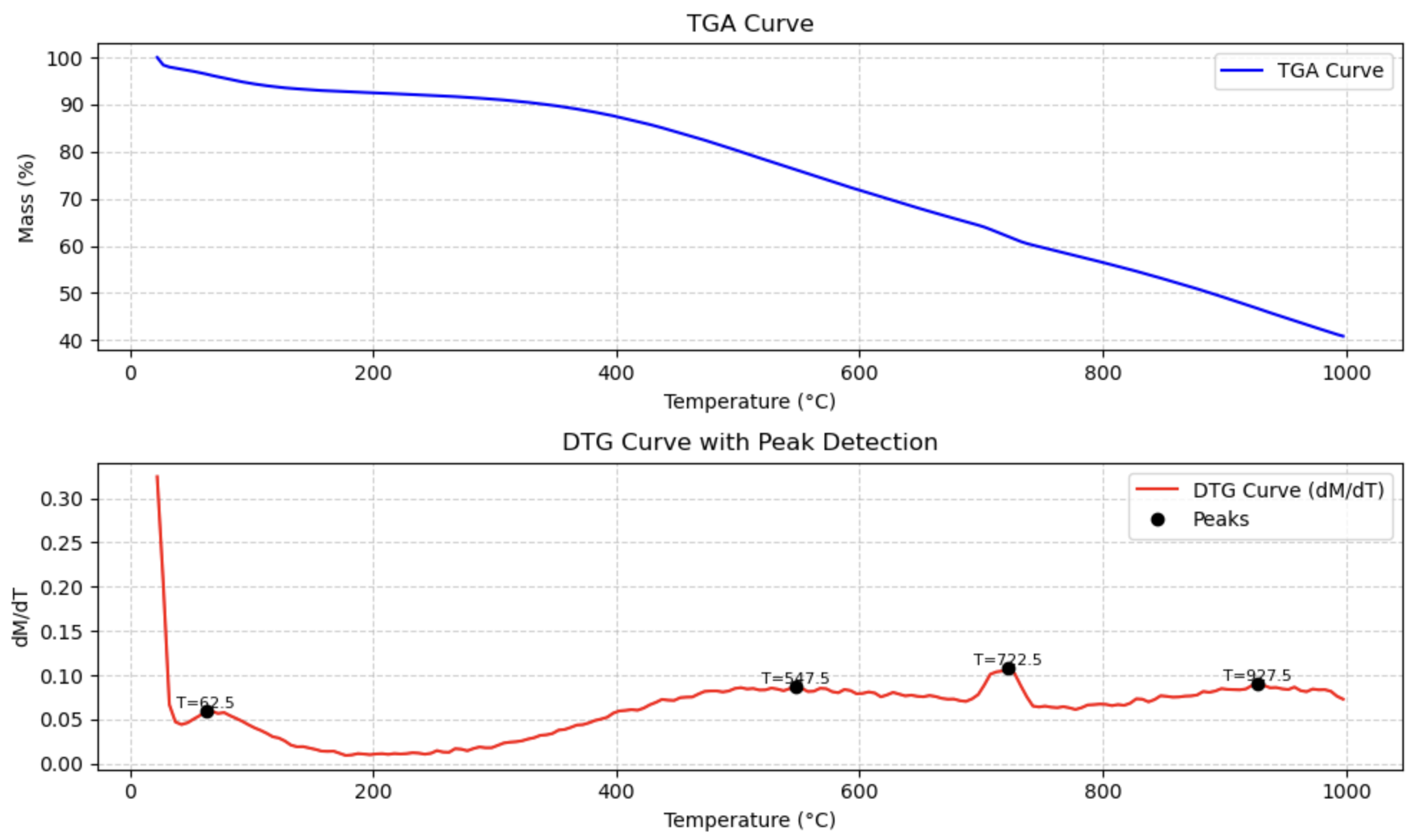
TGA(data, application="kinetics")

7. AI Core — Intelligent Models for Materials Science¶

🌍 Overview¶

In the era of Artificial Intelligence, breakthroughs in science and engineering are increasingly driven by machine learning models that can learn from data, generalize complex patterns, and make predictions faster and more accurately than traditional methods.

Following the revolution of transformer architectures and fine-tuning techniques, modern AI systems — from large language models (LLMs) like GPT to domain-specific predictors — have transformed the way we process information. However, while fields such as natural language processing and computer vision have extensive access to pre-trained and fine-tuned models through platforms like Hugging Face, materials science and nanotechnology have historically lacked such unified AI model repositories.

The AI Core module in PyGamLab was created to close that gap.

⚙️ Purpose and Vision¶

The ai_core module provides a structured and unified framework to access, manage, and utilize pre-trained AI models designed for materials science, solid-state physics, nanotechnology, and chemical engineering.

Instead of spending weeks retraining machine learning models from scratch — searching GitHub for partial implementations, reprocessing data, or manually reconstructing hyperparameters — researchers can now instantly load ready-to-use models stored in the .gam_ai format.

Each model comes with complete metadata, including: - Model name
and architecture
- Training data sources
- Hyperparameter configurations
- Target properties and data types
- Publication or DOI references
- Performance metrics and version history

This makes PyGamLab’s AI Core not only a repository of models, but a knowledge graph of the machine learning landscape in materials science.

🧠 Core Capabilities¶

The AI Core module revolves around two key components:

This class is responsible for loading and managing a saved AI
model.
Each .gam_ai file contains: - Encoded model data (.joblib
format stored as Base64)
- Model metadata (JSON structure)
- Versioning and configuration details

You can easily load a model like this:

from PyGamLab.ai_core import GAM_AI_MODEL

model = GAM_AI_MODEL("cu-nanocomposites-porosity-dt")
model.summary()

This command loads the model, prints its metadata (e.g., dataset size, training source, author, DOI, etc.), and prepares it for predictions. Once loaded, the model object (model.ml_model) behaves like a scikit-learn estimator — meaning you can directly call:

y_pred = model.ml_model.predict(X_test)

This class provides a high-level machine learning pipeline for managing end-to-end workflows — from loading models and metadata to performing predictions, generating plots, and summarizing results. Example usage:

from PyGamLab.ai_core import GAM_AI_WORKFLOW

workflow = GAM_AI_WORKFLOW("cu-nanocomposites-porosity-dt")
workflow.get_GAM_AI_MODEL().summary()

This workflow integrates seamlessly with other PyGamLab modules — such as Data_Analysis and Structures — enabling cross-disciplinary research where you can: Predict material properties (porosity, conductivity, elasticity, etc.) Correlate results with experimental datasets Export and visualize results automatically

📊 Summary Table of AI Core Features¶

Category*	Function / Class	Description*	Example Usage
Model Access	`GAM_AI_MODEL()`	Load and manage a pre-trained model in `.gam_ai` format.	`model = GAM_AI_MODEL( "cu-nano-dt")`
Workflow A utomation	`G AM_AI_WORKFLOW()`	Automate end-to-end ML pipeline (summary, prediction, v isualization).	`workflow = G AM_AI_WORKFLOW( "cu-nano-dt")`
Model Summary	`.summary()`	Display model name, architecture, hy perparameters, source, and metrics.	`mo del.summary()`
P rediction	`.predict(X)`	Predict target properties using pre-trained model.	``y_pred = model.ml_mod el.predict(X)``
Visu alization	` .plot_results()`	Auto-generate plots for predicted vs actual data or feature importance.	`workflow.p lot_results()`
Metadata Access	`.metadata`	Retrieve complete metadata (author, DOI, performance, etc.).	`model.me tadata["doi"]`
Model In tegration	`to_sklearn()` / `from_sklearn()`	Convert between PyGamLab and Scikit-learn models.	`model .to_sklearn()`
E valuation	`.evaluate()`	Compute metrics such as MAE, R², RMSE, etc.	`workf low.evaluate(y_ true, y_pred)`
Model Sharing	`.save_model()` / `.load_model()`	Save or load `.gam_ai` models for sharing and re producibility.	`model.s ave_model("my_m odel.gam_ai")`
Cross-Comp atibility*	Integration with `Data_Analysis` and `Structures`	Link AI predictions to s tructure-based or experimental datasets.	`workflow.link _to_structure(s tructure_obj)`

💡 Why It Matters¶

The AI Core module in PyGamLab is more than just a technical feature — it represents a paradigm shift in how researchers approach artificial intelligence in materials science.

Traditional workflows required: - Manually finding and cleaning
datasets.
- Training models from scratch using custom code.
- Tuning hyperparameters by trial and error.
- Reproducing prior results from incomplete repositories.

This consumed weeks of effort and computing power.

With AI Core, this process becomes instant and transparent:

🔁 Reproducibility — Each model includes versioned metadata, making experiments repeatable and verifiable.
⚡ Speed — Pre-trained models enable immediate predictions, skipping data collection and training stages.
🧩 Interoperability — Works natively with other PyGamLab modules such as data_analysis, structures, and databases.
🧠 Accessibility — Researchers without deep ML knowledge can still perform advanced analysis and prediction.
🌐 Community Growth — Encourages sharing and reusing models across labs and institutions, reducing duplication of effort.

Ultimately, AI Core bridges the gap between AI theory and practical engineering, making machine learning a daily research tool instead of a specialized challenge.

🔮 Future Directions¶

The PyGamLab AI Core will continue to evolve to support: - Graph
Neural Networks (GNNs) for atomic and molecular graph
representation.
- Transformer-based models for material sequence and structure
prediction.
- Active learning loops that continuously refine models as new
data is added.
- Integration with cloud repositories (e.g., Zenodo, Hugging Face,
Materials Cloud) for synchronized model access.
- Interactive dashboards for live visualization and performance
comparison.

Our long-term goal is to make PyGamLab the central ecosystem for intelligent materials discovery —

a place where data, structures, simulations, and AI come together seamlessly.

PyGamLab’s AI Core turns artificial intelligence into a practical companion for scientists and engineers.

Benefit	Impact
Ready-to-use AI Models	Skip training, start predicting immediately.
Standardized Metadata	Ensure research is traceable and reproducible.
Cross-Module Compatibility	Combine AI with data analysis and structure generation.
Scalable Workflows	Handle both small and large datasets with ease.
Open Collaboration	Encourage community-driven model sharing and improvement.

In short — AI Core is where materials science meets machine intelligence.

Example Usage¶

#for starting the workflow you can import the class
from PyGamLab.ai_core import Gam_Ai_Workflow

workflow=Gam_Ai_Workflow(model_name='your_model_name_here')

#so you can see list of available models
#workflow.list_models()
#or at this website
#.....

## Example Usage
#for instance we can use 'cu-nanocomposites-young-modulus-pipe-mlp' model
#Actually it is easy to create workflow object and use its methods
from PyGamLab.ai_core import Gam_Ai_Workflow
workflow=Gam_Ai_Workflow(model_name='cu-nanocomposites-young-modulus-pipe-mlp')

✅ Loaded GAM_AI_MODEL: 'cu-nanocomposites-young-modulus-pipe-mlp'
✅ Loaded model 'cu-nanocomposites-young-modulus-pipe-mlp' (pipe) successfully.

#so first of all you can have summary of the model
workflow.summary()

📘 MODEL SUMMARY
model_name: cu-nanocomposites-young-modulus-pipe-mlp
file_path: /Users/apm/anaconda3/envs/DL/lib/python3.10/site-packages/PyGamLab/ai_core/gam_models/cu-nanocomposites-young-modulus-pipe-mlp.gam_ai
model_type: pipe
description: The presence of vacancy defects in graphene negatively affects the structural behaviors of the composite beams to a certain degree. So, increasing the temperature & defects decrease the mechanical properties, Increasing the percentage of Graphene increase the mechanical properties.
author_name: Shaoyu Zhao, Yingyan Zhang, Yihe Zhang et al.
author_email: None
trainer_name: Ali Pilehvar Meibody
best_accuracy: -0.029005423067057112
doi: https://doi.org/10.1007/s00366-022-01710-w
hyperparam_range: {'model__hidden_layer_sizes': [[50], [100], [100, 50], [100, 100]], 'model__activation': ['relu', 'tanh', 'logistic'], 'model__solver': ['adam', 'lbfgs'], 'model__alpha': [0.0001, 0.001, 0.01], 'model__learning_rate': ['constant', 'adaptive'], 'model__max_iter': [500, 1000]}
best_params: {'model__activation': 'relu', 'model__alpha': 0.01, 'model__hidden_layer_sizes': [100, 100], 'model__learning_rate': 'adaptive', 'model__max_iter': 500, 'model__solver': 'lbfgs'}
ml_model: GridSearchCV(cv=5,
             estimator=Pipeline(steps=[('scaler', MinMaxScaler()),
                                       ('model', MLPRegressor())]),
             n_jobs=-1,
             param_grid={'model__activation': ['relu', 'tanh', 'logistic'],
                         'model__alpha': [0.0001, 0.001, 0.01],
                         'model__hidden_layer_sizes': [(50,), (100,), (100, 50),
                                                       (100, 100)],
                         'model__learning_rate': ['constant', 'adaptive'],
                         'model__max_iter': [500, 1000],
                         'model__solver': ['adam', 'lbfgs']},
             return_train_score=True,
             scoring='neg_mean_absolute_percentage_error')

#you can see what is file path , name of mdoel
#what is type of model
#description of data and doi of article
#and best acuracy and also model
#for extracting the model you can just use this method

gam_ai_model=workflow.get_GAM_AI_MODEL()

#you can see the type of that

print(type(gam_ai_model))

<class 'PyGamLab.ai_core.gam_ai.GAM_AI_MODEL'>

#also we have another class named GAM_AI_MODEL
#for importing that you can use this
#from PyGamLab.ai_core import GAM_AI_MODEL
#for now it has only summary but a lot of attributes
#for instance

print('doi:',gam_ai_model.doi)

doi: https://doi.org/10.1007/s00366-022-01710-w

print('description:',gam_ai_model.description)

description: The presence of vacancy defects in graphene negatively affects the structural behaviors of the composite beams to a certain degree. So, increasing the temperature & defects decrease the mechanical properties, Increasing the percentage of Graphene increase the mechanical properties.

#and finally you can extract sklearn model only with

sklearn_model=gam_ai_model.ml_model

print(type(sklearn_model))

<class 'sklearn.model_selection._search.GridSearchCV'>

#so come back to workflow class
#we have talked about gam_ai_model which is from workflow.get_GAM_AI_MODEL() method
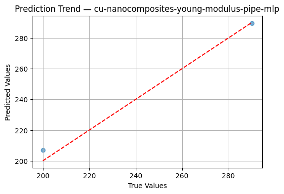
#now we canu use workflow to evaluate its performance
#it is enough to use evaluate() method
import numpy as np

x=np.array([[10, 5.0, 0.5],
            [20, 7.5, 0.8]])
y=np.array([200.0, 290.0])

workflow.evaluate_regressor(x,y)

📈 R²: 0.9884
📉 MAE: 3.5745
📉 MSE: 23.4737

#also you can use predict or you can use refit
#but it is better to see the hypeparameter range

Appendix A: Working with NumPy¶

NumPy is the foundation of scientific computing in Python.

It provides a fast, efficient way to work with large numerical datasets, matrices, and arrays, which are essential for simulations, AI models, and material data analysis.

🌱 What is NumPy?¶

NumPy (short for Numerical Python) adds powerful array objects and mathematical functions to Python.

It replaces slow Python loops with optimized C-based operations that make it incredibly fast.

In PyGamLab, NumPy is used behind the scenes for almost everything — from handling structure coordinates to performing physical calculations and data transformations.

🔢 Creating Arrays¶

import numpy as np

# Create simple arrays
a = np.array([1, 2, 3])
b = np.array([[1, 2, 3], [4, 5, 6]])

print(a.shape)  # (3,)
print(b.shape)  # (2, 3)

You can also create arrays with predefined values:

np.zeros((2, 3))       # 2x3 array filled with zeros
np.ones((3, 3))        # 3x3 array of ones
np.eye(4)              # 4x4 identity matrix
np.arange(0, 10, 2)    # Array from 0 to 10 with step 2
np.linspace(0, 1, 5)   # 5 equally spaced values between 0 and 1

⚙️ Array Operations¶

NumPy allows element-wise operations, which are both fast and easy to read:

x = np.array([1, 2, 3])
y = np.array([10, 20, 30])

print(x + y)  # [11 22 33]
print(x * y)  # [10 40 90]
print(np.sqrt(y))  # [3.16 4.47 5.47]

🔍 Useful Array Methods¶

a = np.random.rand(5, 5)

print(a.mean())      # Average of all elements
print(a.max())       # Maximum value
print(a.min())       # Minimum value
print(a.sum(axis=0)) # Sum of columns
print(a.T)           # Transpose

🧩 Summary Table: NumPy Essentials¶

Step	Task	Function / Method	Description	Example
1*	Im port Num Py	` import numpy as np`	Imports the NumPy library	`` import num py as np``
2*	Cr eate Arra ys	`np.array()`, `np.zeros()`, `np.ones()`, `np.arange()`	Creates arrays of different shapes and values	`arr = n p.array([1 , 2, 3])`
3*	A rray Attr ibut es	`.shape`, `.dtype`, `.size`	Provides information about the array	`a rr.shape`
4*	Inde xing & S lici ng	`[ ]`	Access elements or subarrays	`` arr[0:2]``
5*	Math emat ical Oper atio ns	`np.add()`, `np.mean()`, `np.std()`, `np.dot()`	Performs fast numerical operations	`np.m ean(arr)`
6*	Br oadc asti ng	Implicit operation	Applies arithmetic between arrays of different shapes	` arr + 5`
7*	Ra ndom N umbe rs	`np.random.rand()`, `` np.random.randint()``	Generates random data	`np .random.ra nd(3, 3)`
8*	Res hape Arra ys*	`.reshape()`	Changes the shape of arrays without changing data	` arr.resha pe(2, 3)`
9*	Save & Lo ad	`np.save()`, `np.load()`	Saves and loads arrays efficiently	`np.save ('array.np y', arr)`
10	Int egra tion with Py GamL ab*	Arrays as input data	Used for materials data, coordinates, and simulations	``gam _structure = pygamla b.Structur e(np.array ([…]))``

✅ In short:

NumPy is the backbone of scientific computing — providing fast array operations and mathematical tools that power nearly every PyGamLab function.

Further Learning¶

NumPy Official Docs: https://numpy.org/doc Focus on learning indexing, slicing, and broadcasting — they are the heart of efficient data handling.

Appendix B: Working with Pandas¶

Pandas is your best friend when dealing with structured data — CSV files, Excel sheets, database outputs, or any tabular dataset.

It is built on top of NumPy and provides two main data structures: - Series → One-dimensional labeled array (like a single column) - DataFrame → Two-dimensional labeled table (like an Excel sheet)

In PyGamLab, Pandas is used everywhere — especially in the data_analysis and databases modules — to load, clean, and process experimental and simulation data.

🌱 What is Pandas?¶

Pandas makes working with data much easier by allowing: - Fast reading/writing of files (CSV, Excel, SQL, JSON) - Easy data filtering, grouping, and summarizing - Seamless integration with NumPy, Matplotlib, and scikit-learn

Whenever you have data in rows and columns, think Pandas.

📥 Reading Data¶

The first step is usually importing your data.

Pandas can read from almost any source — the most common being CSV and Excel.

import pandas as pd

# Read a CSV file
data = pd.read_csv("sample_data.csv")

# Read an Excel file
data_excel = pd.read_excel("data.xlsx", sheet_name="Sheet1")

# Display the first five rows
print(data.head())

You can also load directly from a URL or database connection.

📊 Basic Operations¶

Once your data is loaded, you can explore and manipulate it easily:

print(data.columns)     # Show column names
print(data.info())      # Summary of dataset
print(data.describe())  # Basic statistics for numeric columns

Select a column or filter rows:

temperatures = data["Temperature"]
filtered = data[data["Pressure"] > 10]

# Create a new calculated column
data["Density_Ratio"] = data["Density"] / data["Temperature"]

Rename columns for clarity:

data = data.rename(columns={"Temp": "Temperature"})

🔄 Saving Processed Data¶

After cleaning or analyzing your dataset, you can save it back to a file:

data.to_csv("processed_data.csv", index=False)
data.to_excel("output.xlsx", sheet_name="Results", index=False)

🧾 Summary Table: Pandas for Data Handling¶

Step	Task	Function / Method	Description	Example
1*	Im port Pand as	`` import pandas as pd``	Imports the Pandas library	`i mport pand as as pd`
2*	Cr eate Dat aFra me	`pd.DataFrame()`	Creates a table-like structure with rows and columns	`df = pd.DataFra me(data)`
3*	Read Da ta	`pd.read_csv()`, `pd.read_excel()`	Loads data from external files	`` df = pd.re ad_csv(‘da ta.csv’)``
4*	View Da ta	`df.head()`, `df.tail()`	Displays the first or last few rows	`d f.head()`
5*	Ins pect Da ta*	`df.info()`, `df.describe()`	Shows structure and summary statistics	`df.de scribe()`
6*	Se lect Col umns / Ro ws	`df['col']`, `df.loc[]`, `df.iloc[]`	Access subsets of data	`` df.loc[0, ‘value’]``
7*	Fi lter Da ta	Boolean indexing	Filters based on conditions	`df [df['value '] > 10]`
8*	G roup & Agg rega te	`df.groupby()`, `.mean()`, `.sum()`	Groups data and calculates statistics	`df.grou pby('type' ).mean()`
9*	Ha ndle Mis sing Valu es	`df.dropna()`, `df.fillna()`	Removes or replaces missing data	`df.f illna(0)`
10	Ex port Da ta	`df.to_csv()`, `df.to_excel()`	Saves data to files	`df.to _csv('outp ut.csv')`

✅ In short:

Pandas is your go-to library for loading, cleaning, and analyzing materials data — it forms the foundation of PyGamLab’s data_analysis module and is essential for preparing inputs for AI models. — ## 📘 Further Learning Official Docs: https://pandas.pydata.org/docs

Table of Contents¶

0. Overview of PyGamLab¶

Key Features¶

How This Tutorial Helps You¶

1. How to Install¶

Step 1: Open Your Command Line Interface¶

Step 2: Install PyGamLab¶

Step 3: Verify the Installation¶

Installing pip (if needed)¶

2. Constants & Converters¶

Why Constants & Converters Matter¶

How PyGamLab Implements This¶

Example Usage¶

3. Functions¶

What is the Functions Module?¶

Purpose of the Functions Module¶

Advantages of Using the Functions Module¶

Examples of Functions and Usage¶

4. Structures¶

Advantages of the Structures Module¶

Submodules Overview¶

Example Usage¶

5. Databases¶

Why Access to Databases Matters¶

Supported Databases¶

The Challenge of Using Multiple Databases¶

PyGamLab’s Unified Solution: Explorer¶

Advantages of the Databases Module¶

Example Usage¶

6. Data Analysis¶

Why PyGamLab’s Data Analysis Module?¶

Core Design Philosophy¶

How It Works¶

Example: Analyzing NMR Data¶

Example: Analyzing XPS Data¶

DSC¶

TGA¶

7. AI Core — Intelligent Models for Materials Science¶

🌍 Overview¶

⚙️ Purpose and Vision¶

🧠 Core Capabilities¶

📊 Summary Table of AI Core Features¶

💡 Why It Matters¶

🔮 Future Directions¶

Example Usage¶

Appendix A: Working with NumPy¶

🌱 What is NumPy?¶

🔢 Creating Arrays¶

⚙️ Array Operations¶

🔍 Useful Array Methods¶

🧩 Summary Table: NumPy Essentials¶

Further Learning¶

Appendix B: Working with Pandas¶

🌱 What is Pandas?¶

📥 Reading Data¶

📊 Basic Operations¶

🔄 Saving Processed Data¶

🧾 Summary Table: Pandas for Data Handling¶

PyGamLab’s Unified Solution: `Explorer`¶